the Creative Commons Attribution 4.0 License.
the Creative Commons Attribution 4.0 License.
 | 28 Feb 2019
Sensor characterization by comparative measurements using a multi-sensor measuring system
Sebastian Hagemeier
Markus Schake
Peter Lehmann
Typical 3-D topography sensors for the measurement of surface structures in the micro- and nanometre range are atomic force microscopes (AFMs), tactile stylus instruments, confocal microscopes and white-light interferometers. Each sensor shows its own transfer behaviour. In order to investigate transfer characteristics as well as systematic measurement effects, a multi-sensor measuring system is presented. With this measurement system comparative measurements using five different topography sensors are performed under identical conditions in a single set-up. In addition to the concept of the multi-sensor measuring system and an overview of the sensors used, surface profiles obtained from a fine chirp calibration standard are presented to show the difficulties of an exact reconstruction of the surface structure as well as the necessity of comparative measurements conducted with different topography sensors. Furthermore, the suitability of the AFM as reference sensor for high-precision measurements is shown by measuring the surface structure of a blank Blu-ray disc.


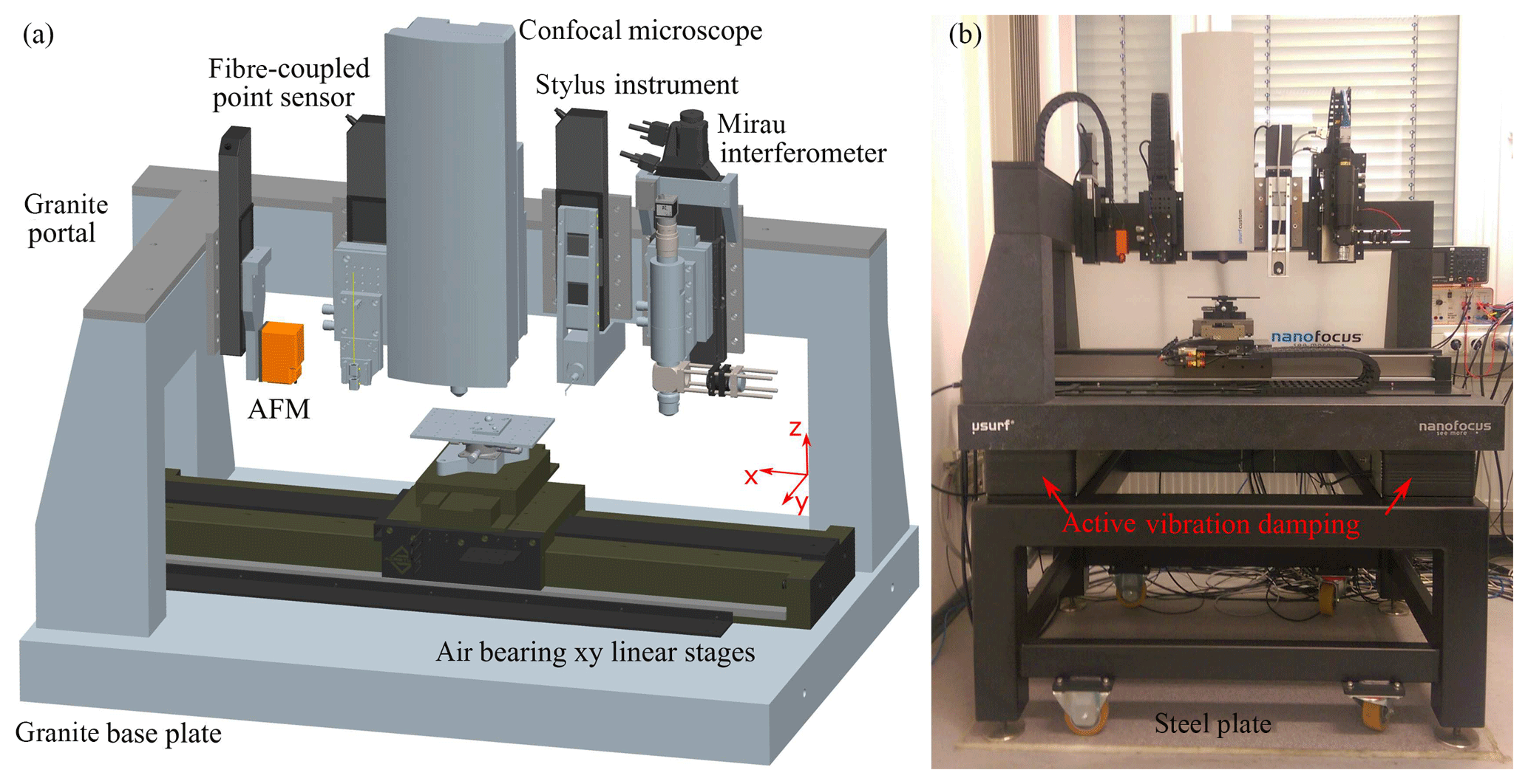
Figure 1Schematic representation of the multi-sensor measuring system with five different topography sensors (a) and a photograph of the measuring system with active vibration damping on a steel plate reducing mechanical environmental vibrations (b).
The characterization of surface structures in the micro- and nanometre range can be done by various types of topography sensors. The demands on topography sensors with regard to accuracy and measurement speed increase steadily. Currently the best-known method for three-dimensional topography measurement with respect to its transfer behaviour is the tactile stylus method, where the surface of the specimen is scanned with a stylus tip. However, the tip may influence the sample to be measured and also limits the measuring speed typically up to 1 mm s−1. Therefore, there are efforts to increase the measuring speed of tactile sensors and to reduce the wear of the stylus tip (Morrison, 1996; Doering et al., 2017). Doering et al. (2017) present a microprobe which allows tactile roughness measurements with a lateral scanning speed of 15 mm s−1.
Optical methods such as confocal microscopy, coherence scanning interferometry (CSI) and laser interferometry provide an alternative (Jordan et al., 1998; de Groot, 2015; Schulz and Lehmann, 2013). The advantage of these methods is a fast and contactless measurement of the surface topography. Damages of the measuring surface as well as maintenance costs and measuring deviations due to worn probe tips are eliminated. For the compensation of disturbances caused by external vibrations, different methods exist (Tereschenko et al., 2016; Seewig et al., 2013; Kiselev et al., 2017; Schake and Lehmann, 2018). However, depending on the surface topography, more or less systematic measurement errors may also occur. Examples are artefacts known as batwings (Harasaki and Wyant, 2000; Xie et al., 2017), phase jumps resulting from the slope effect in white-light interferometry (Lehmann et al., 2016) and also laser interferometry (Schake et al., 2015), artefacts from crosstalk between neighbouring pinholes of a spinning disc of a confocal microscope (Fewer et al., 1997), and artefacts occurring by equal curvature of the wavefront and the measuring surface (Mauch et al., 2012). For an investigation of these effects it is necessary to distinguish between the real and the measured surface. Therefore, measurements are performed on specimens with a known surface structure like a surface standard or by comparing the measurement results with those of a reference sensor. An advantage of comparative measurements with reference sensors in the same system configuration is the feasibility of measurement of arbitrary surface structures under identical environmental conditions. For this purpose a multi-sensor measuring system has been developed in our lab (Hagemeier and Lehmann, 2018a). Next to the investigation of different systematic effects it is possible to characterize the transfer behaviour of our self-assembled topography sensors with this measuring system. A similar multi-sensor concept has already been pursued by Wiedenhöfer (2011) and Weckenmann (2012). However, here the priority targets were the extension of the measuring range and the coverage of metrological requirements for different measuring objects through the use of different optical and tactile sensors.
The multi-sensor measuring system comprises two self-assembled optical sensors (a Mirau interferometer and a fibre-coupled interferometric point sensor) as well as three commercial sensors (an atomic force microscope, AFM; a confocal microscope; and a tactile stylus instrument). The sensors are mounted on an L-shaped granite portal as shown in Fig. 1. Each sensor is connected to the granite portal by a vertically aligned linear stage. The linear stages provide a vertical positioning of each sensor in a range of 100 mm. With two horizontally aligned air bearing linear stages it is possible to position a specimen in the measuring volume of the respective sensor. A lateral measurement field of 150 mm × 100 mm is covered by all topography sensors for comparative measurements. In addition, the xy linear stages are used as scan axes for scanning a specimen surface horizontally as well as for stitching of several measurement fields. The repeatability of the xy linear stages is denoted by ±400 nm in the x direction and ±50 nm in the y direction. Based on this positioning accuracy it is possible to measure surfaces with stochastic structures without a reference point.
In order to compensate for environmental vibrations, several techniques are employed. At higher frequencies vibrations are damped by the inertial mass of the granite used and the lower frequency spectrum is covered by an active vibration damping system shown in Fig. 1b.
The atomic force microscope (AFM) can measure the surface in the tactile static mode and the contactless dynamic mode. In the more precise dynamic mode the maximum rms value of the noise of the measured height values is specified by 150 pm. The lateral deflection of the cantilever via three internally installed coils results in a maximum diamond-shaped measuring field of 110 µm × 110 µm and a square field of 79 µm × 79 µm. The maximum vertical deflection of the cantilever is 22 µm. Besides the low noise of the height values the lateral resolution of this sensor is much better than the resolution of optical sensors based on microscopic imaging, as demonstrated by measuring the surface of a Blu-ray disc in Sect. 3. For this reason, the AFM generates a precise surface topography of the structures to be measured and thus is qualified as a precision reference sensor for optical topography sensors.
A further reference sensor is the confocal microscope. A rotating multi-pinhole disc generates the confocal effect by filtering the light of an LED light source and the light field in the image plane. During one rotation a complete image of the surface to be measured is detected by an areal CCD camera. The depth scan required for the topography measurement is done by changing the distance between the microscope objective and specimen by a stepwise motion of the objective using a piezoelectric-driven stage. At each step the camera detects an image of the surface. The confocal sensor provides a measurement field of 320 µm × 320 µm by a total magnification of 23. At a numerical aperture (AN) of 0.95 the lateral optical resolution is approximately 320 nm using the Rayleigh criterion for conventional optical microscopy. By the confocal effect the lateral optical resolution is improved compared to classical light microscopy (Sheppard and Choudhury, 1977; Xiao et al., 1988; Wilson, 1990). As a result of the optical magnification and the pixel pitch of the camera the lateral sampling interval in the object plane is approximately 320 nm. Based on the Shannon criterion, grating structures with a period larger than 640 nm can be reconstructed. The vertical resolution is specified with a noise level of 2 nm. To obtain an overview of the surface to be measured it is possible to generate conventional microscopic images besides the confocal measurement mode. Due to the high AN and the different working principle compared to interferometric sensors, the confocal microscope is an appropriate optical reference sensor.
The third reference sensor is the tactile stylus instrument. In particular, tactile measurements of surface contour and roughness can be obtained with this sensor. A stylus tip is brought into contact with the surface of the specimen and scans a line of 26 mm in the y direction with a scan velocity in a range of 0.1 to 1 mm s−1 (for the coordinates see Fig. 1). Height differences of the surface structure result in deflection of the tip which is measured. In combination with the x axis, several parallel profiles can be scanned and combined to a 3-D topography. The accuracy of the measured height information is specified by the residual value Rz0 according to DIN EN ISO (3274); see Table 1.
Table 1Scanning speed values and related Rz0 according to DIN EN ISO (3274), Lc = 0.25 mm, Lc ∕ Ls = 100.
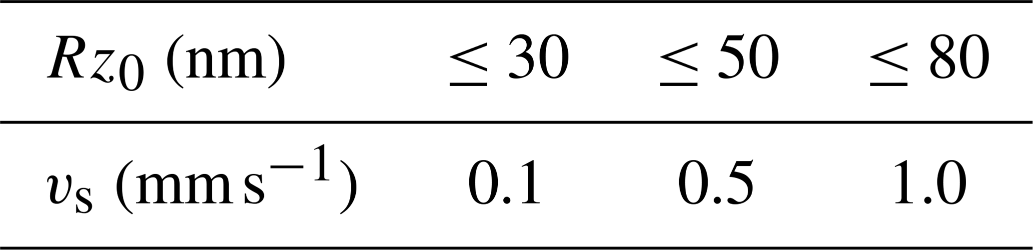
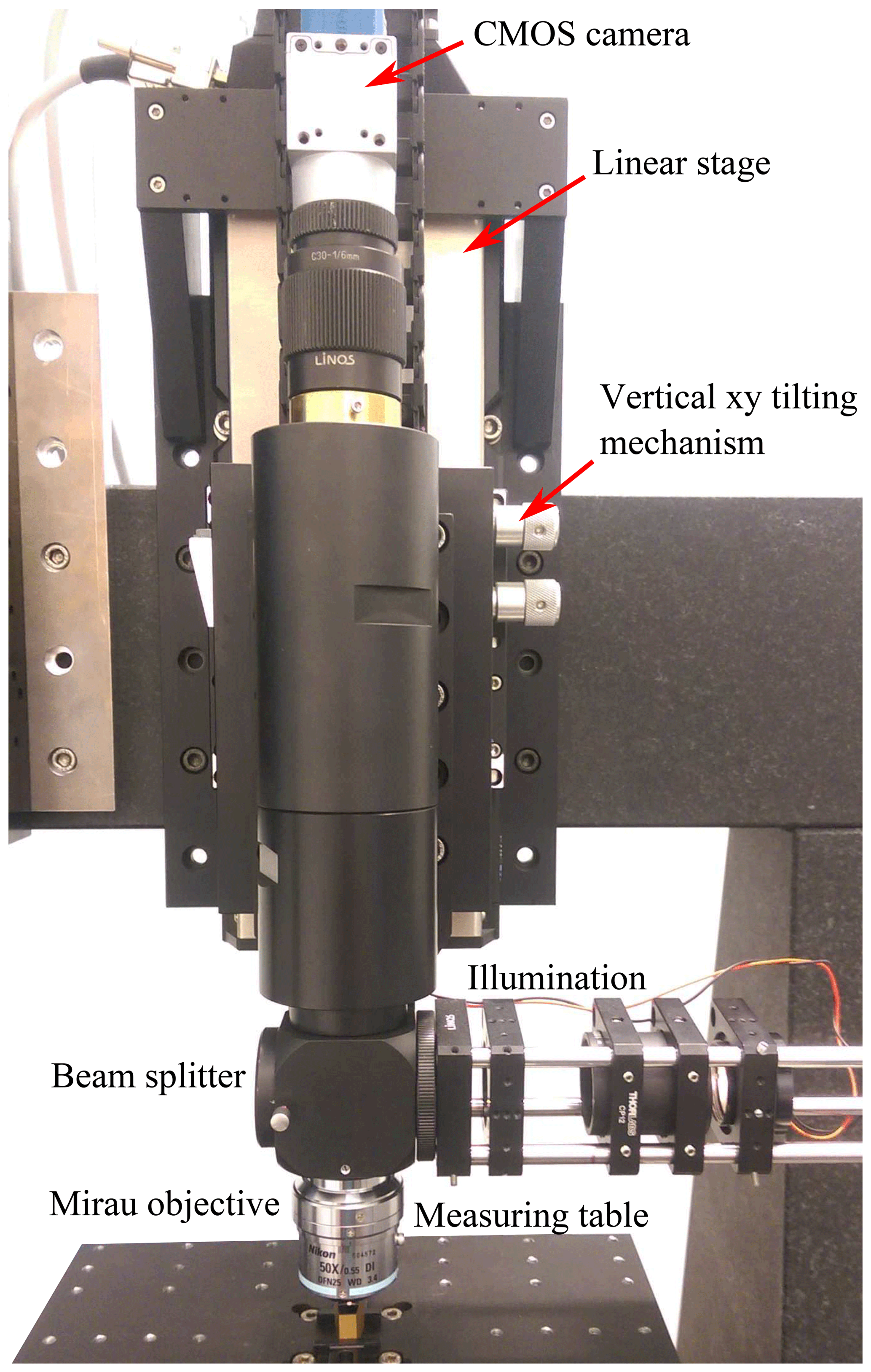
Figure 2Self-assembled Mirau interferometer measuring a chirp standard provided by Physikalisch-Technische Bundesanstalt (PTB).
In addition to the three reference sensors, two different self-assembled interferometric topography sensors are integrated in the multi-sensor system. One of these 3-D sensors is the Mirau interferometer shown in Fig. 2. With this interferometer the transfer characteristics of white-light interferometers are investigated as an example, including the investigation of artefacts like the batwing effect (Xie et al., 2016, 2017). A special feature of this Mirau interferometer is its ability to simply adapt the spectral characteristics of the light source and to perform depth scans of up to 100 mm using a stepper-motor-driven linear axis instead of an additional piezo-driven positioning system. Using a linear depth scan in combination with a CMOS camera with a USB3.0 interface, high-speed measurements are possible. At full resolution (2048 pixels × 2048 pixels) the camera captures 90 frames per seconds (fps) or 360 fps with a resolution of 512 pixels × 2048 pixels. For signal analysis different algorithms are used. In addition to the determination of the height values by detecting the position of the envelope, the more precise phase evaluation is inter alia obtained by a lock-in algorithm (LT algorithm) or frequency domain analysis (Tereschenko, 2018; de Groot et al., 2002).
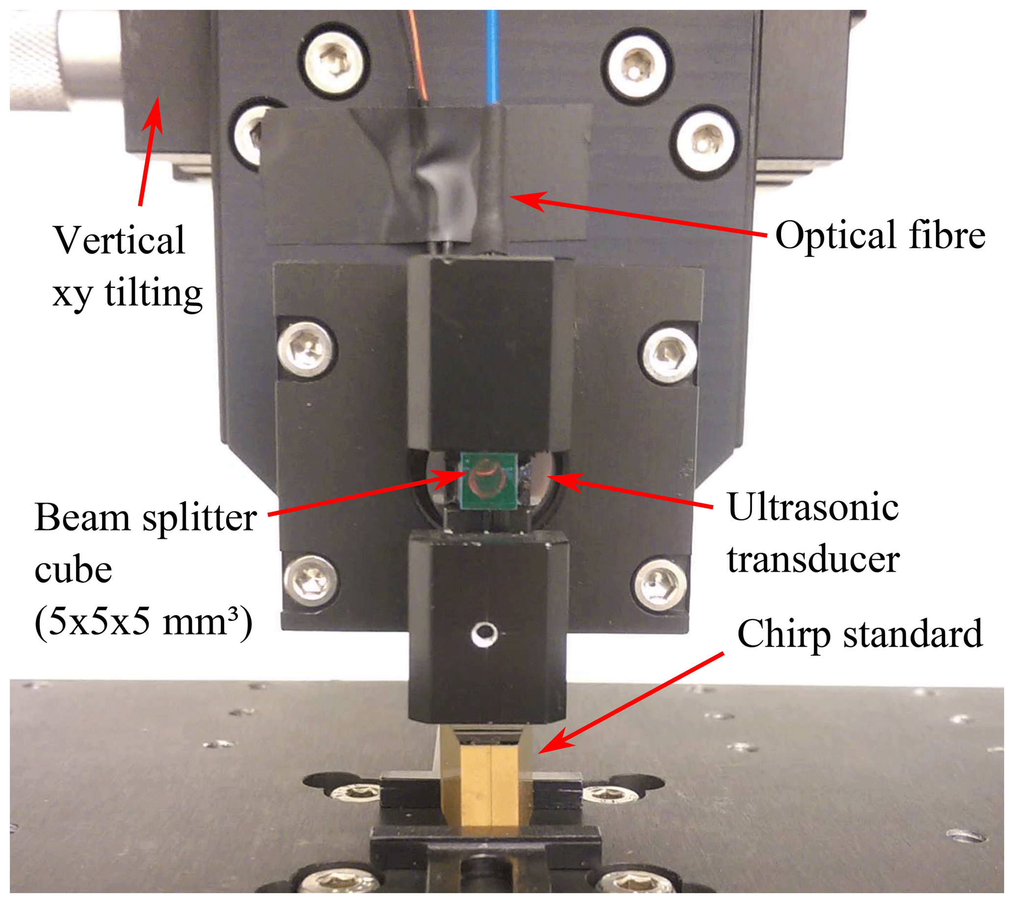
Figure 3Fibre-coupled interferometric–confocal high-speed distance sensor using a 1550 nm laser source.
Figure 3 shows the practical realization of a fibre-coupled interferometric–confocal high-speed sensor (Schulz and Lehmann, 2016). The fundamental principle of this sensor is based on a Michelson interferometer. A laser beam with a wavelength λL of 1550 nm propagating from the end face of the optical fibre is divided by a beam splitter in a measurement and a reference beam with the intensities Im and Ir. The modulation of the optical path length by an ultrasonic transducer, which actuates the reference mirror, allows a phase detection to calculate the height value h(x,y). Neglecting the offset, the two-beam interference equation takes the form
Here and fa represent the amplitude and frequency of the oscillating reference mirror. For each period of the oscillating mirror, two height values result. Therefore, the oscillation frequency fa of 58 kHz used yields 116 000 height values per second. This high acquisition rate allows a movement speed of the horizontal scan axis up to 100 mm s−1 as demonstrated using a sinusoidal standard (Hagemeier and Lehmann, 2018a). However, if a lower scan velocity is used, the high acquisition rate can be utilized to filter and improve the accuracy of the height values. In order to generate a 3-D topography of the surface to be measured, the air bearing xy linear stages are used as scan axes. With AN of approximately 0.4, the lateral resolution is about 2.3 µm according to the Rayleigh criterion. However, the single-mode optical fibre acts as a pinhole of a confocal microscope (Kimura and Wilson, 1991; Gu and Sheppard, 1991; Dabbs and Glass, 1992), improving the lateral resolution and suppressing stray light.

Figure 4Topography and profile of a blank Blu-ray disc measured with the AFM (Hagemeier and Lehmann, 2018b).
At first, the result of a topography measurement on a blank Blu-ray disc (Verbatim BD-RW SL 25 GB) measured by the AFM is presented to underpin the suitability of this instrument as a high-resolution reference sensor. Figure 4 shows the measured topography as well as a 2-D profile of the structure. The tracks of the Blu-ray disc with trapezoidal grooves are well-resolved. The measured track pitch of 324 nm and groove depth of 24 nm correspond to the reported values of 320 and 20 nm (Meinders et al., 2006; Blu-ray Disc Association, 2018; Lin et al., 2006). In order to be able to resolve this fine surface structure, the cantilever EBD-HAR made of HDC/DLC (high-density carbon/diamond-like carbon) by Nanotools is used. With an opening angle below 8∘ this cantilever is particularly suitable for measurements of steep edges and fine structures. The air bearing xy linear axes were also lowered prior to the measurement in order to minimize the influence of vibrations caused by the air stream. For comparison, a high-resolution Linnik interferometer with a AN of 0.9 and a blue LED light source with a centre wavelength of 460 nm resolves the tracks of the disc too but not as detailed as the AFM (Lehmann et al., 2018).
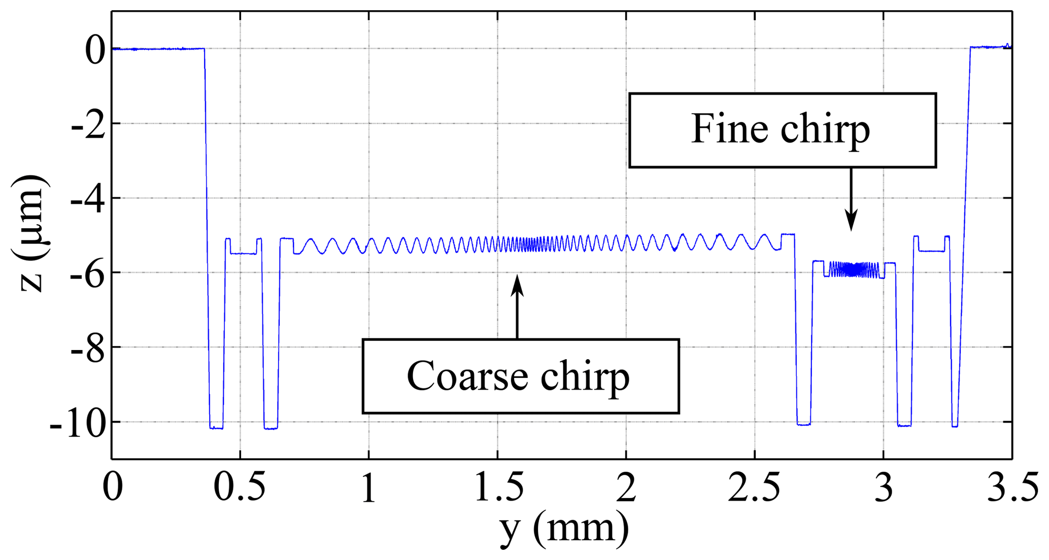

Figure 6Profiles of the fine chirp structure obtained by various topography sensors: (a) 50× Mirau interferometer with a AN of 0.55 (phase evaluation using the LT algorithm) and a central wavelength of 590 nm, (b) unwrapped profile from (a), (c) confocal microscope, (d) high-speed sensor with two different scan velocities (blue: 0.1 mm s−1; red: 1 mm s−1), (e) AFM with a Tap190Al-G cantilever and (f) contact stylus instrument with a scan velocity of 0.5 mm s−1 by using a probe according to DIN EN ISO 3274 (2 µm tip radius and an aperture angle of 60∘).
In order to show the necessity of comparison measurements with various topography sensors, measurement results of these sensors are juxtaposed using a chirp structure manufactured by PTB (Physikalisch-Technische Bundesanstalt, Germany). An overview of the surface structure of the chirp standard results from the profile measured by the tactile stylus instrument; see Fig. 5. The standard is divided into a coarse and a fine chirp structure. Both sinusoidal microstructures are specified with a peak-to-peak amplitude of 400 nm. In the case of the coarse chirp the spatial wavelengths are in a range of 91 to 10 µm and in a range of 12 to 4.3 µm for the fine chirp (Brand et al., 2016). Such a chirp calibration standard can be used to describe the transfer behaviour at different spatial wavelengths (Krüger-Sehm et al., 2007; Seewig et al., 2014). To represent the measured amplitude as a function of the spatial wavelength, the so-called instrument transfer function (ITF) can be used (de Groot and de Lega, 2006). With the knowledge about the real structure, the transfer function is estimated.
Figure 6a shows the measurement result of the Mirau interferometer with AN of 0.55 and a magnification of 50×. In addition to the chirp structure, artefacts occur at the steepest slopes of the structure. These artefacts are phase jumps caused by height displacements occurring as a result of envelope evaluation, which in turn results from a too-low lateral resolution related to low-pass filtering of the fringes (Lehmann et al., 2016). By unwrapping this profile the phase jumps are removed as presented in Fig. 6b. This effect does not appear in the result of the confocal microscope, as it is shown in Fig. 6c. However, the profile indicates a stronger low-pass filtering of the structure compared to the Mirau interferometer. When looking at the profiles, it is striking that there is only a one-sided constriction of the profile at the centre. In theory, double-sided constrictions are to be expected in a low-pass-filtered profile. A possible reason for this effect is indicated by an AFM measurement. Figure 6e shows the chirp profile measured by the AFM in the dynamic mode using a Tap190Al-G cantilever from BudgetSensors. Again, there is also a one-sided constriction with a height reduction of approx. 40 nm. In addition, the upper peaks of the sinusoidal structure in the centre of the chirp standard are tapered, resulting in a sharp-combed chirp structure. Therefore, the top levels are more affected by low-pass filtering compared to the bottom levels. To achieve high accuracy in the determination of the transfer behaviour of a topography sensor, the profile measured by AFM can be used as a reference representing the original course of the chirp structure.
In the further three subsections the transfer behaviour of the tactile stylus instrument, the fibre-coupled high-speed sensor and the confocal microscope is investigated in more detail.
3.1 Tactile stylus instrument
For the measurement of the fine chirp structure with the tactile stylus instrument, a probe with a 2 µm tip radius and a cone angle of 60∘ according to DIN EN ISO (3274) is used. Compared to the lateral resolution of the interferometric high-speed sensor (see Fig. 6d), similar low-pass filtering of the measured chirp structure is expected. However, the measured stylus profile in Fig. 6f shows a fairly good reproduction of the reference structure. Deviations to the structure measured by the AFM are inter alia formed by the lateral sampling distance of 0.5 µm, measuring deviations given by the residual value up to 50 nm according to Table 1 and the dilatation coming from the stylus tip. Due to the mechanical contact of the tip and the surface to be measured, no low-pass filtering of the upper tapered peaks appears and the real shape is reproduced nearly correctly.
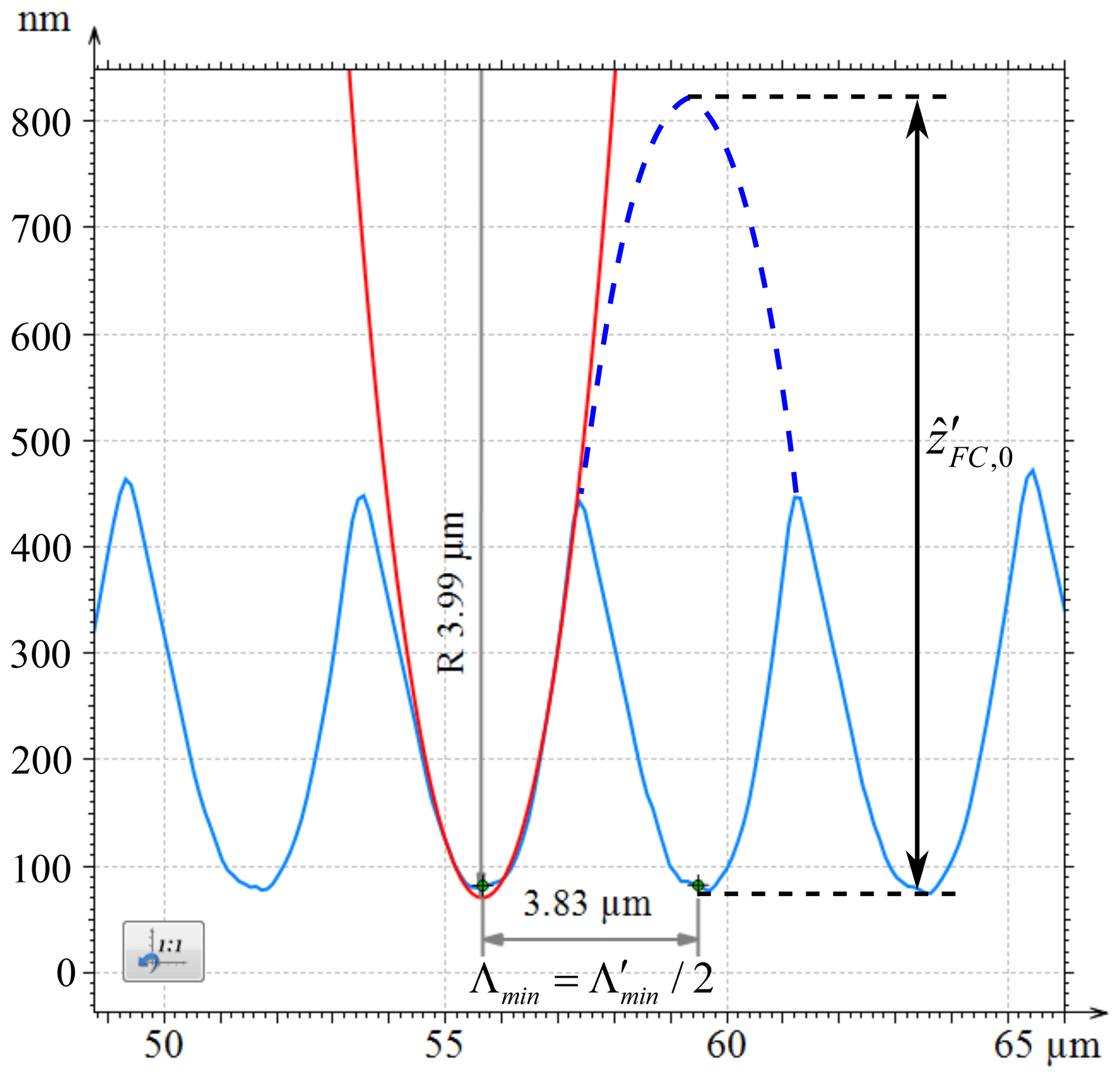
Figure 7Section of the chirp profile with the shortest spatial wavelength measured by the AFM (blue line) and a fitted concentric circle (red line) with a radius of 3.99 µm, using the software MountainsMap. The additional blue dashed line illustrates a sine with the spatial wavelength and the amplitude .
The radius of curvature RFC,min at the smallest spatial wavelength Λmin of the nominal sinusoidal chirp structure is
where Λmin=3.8 µm (see Fig. 7) and the amplitude is equal to 200 nm. Because the structure is sharp-combed instead of sinusoidal, the radius of curvature of the grooves is assumed to be reasonably greater than 1.83 µm. This assumption is confirmed by the reference measurement of the AFM plotted in Fig. 7. Next to the area of the smallest spatial wavelengths (blue curve), a fitted concentric circle with a radius of 4 µm (red curve) is depicted, which was created using the analysis software MountainsMap. An explanation for the difference between the calculated value of 1.83 µm and the empirically determined value of 4 µm is given by the sharp-combed structure. The sharp-combed profile almost resembles a rectified sine function of twice the period of the nominal sinusoidal chirp structure. Thus, the period of the sine to calculate the radius corresponds to twice the period Λmin with twice the amplitude:
as it is graphically illustrated by the dashed blue line in Fig. 7. Hence, the grooves can be measured using a stylus instrument with a tip radius of 2 µm. In the case of an optical sensor, low-pass filtering of the structure occurs due to the limited lateral-resolution capabilities, resulting in a double-sided constriction as a simulation shows (Schulz and Lehmann, 2016). On the other hand, when using a tactile measuring method, a one-sided constriction of the grooves is to be expected, because the intrusion between two peaks is first limited before the peaks are no longer resolvable.
In all measured profiles, the smallest period of the chirp structure is 3.8 µm. This leads to the conclusion that there is a deviation from the nominal sinusoidal structure of the 4.3 µm period.
3.2 Optical high-speed sensor
Median filtered profiles of the fine chirp structure obtained by the high-speed sensor with two different lateral scan velocities (blue: 0.1 mm s−1; red: 1 mm s−1) are shown in Fig. 6d. Higher scan velocities such as 80 mm s−1 are also possible as presented by Hagemeier et al. (2019). Both profiles of the high-speed sensor show a similar but stronger low-pass filter effect than the profile of the confocal microscope. In the profile measured at a higher scanning speed there is a stronger low-pass-filtering effect, which is due to an additional averaging over the surface heights caused by the scanning motion. The sawtooth-like structure of both profiles is probably the result of a maladjusted sensor and needs further investigation.
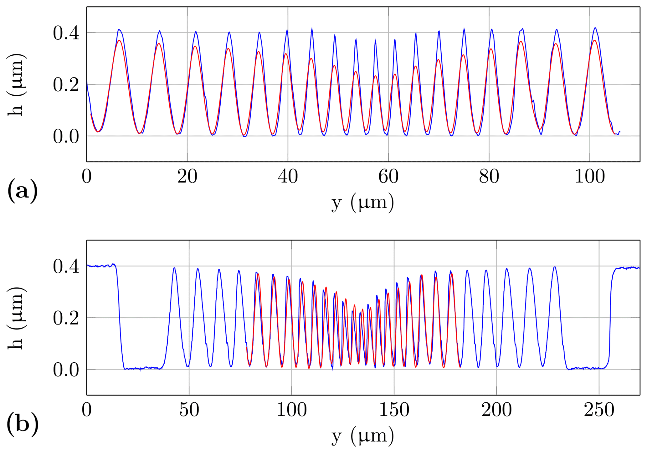
Figure 8Comparison of different profiles of the fine chirp structure: (a) profile measured by AFM (blue) and the same profile filtered with a sliding average filter based on a rectangular impulse response function with a pulse width of 1.85 µm (red), and (b) comparison of the filtered profile (red) from (a) and the structure measured by the interferometric high-speed sensor (blue).
In order to demonstrate the suitability of the measurement results of the AFM as a reference for the characterization of the transfer behaviour of the optical sensors, a simple example is presented in Fig. 8. To simulate the low-pass-filtering effect of the optical sensors a sliding average filter convolving the profile with a rectangular function is used:
with the sampling interval Δy, and a window length of the filter Nw∈ℕ, ny∈ℕ and
Employing the low-pass filtering according to Eq. (4) to hafm, with different parametrization of the minimum beam waist, yields the best match for a width of the rectangular function of NwΔy=1.85 µm shown in Fig. 8a. Through the comparison of this filtered structure with the profile measured by the interferometric high-speed sensor, a good congruence is observed, especially for the constriction of the upper and lower peaks; see Fig. 8b. A mathematical description of the focused laser beam of the high-speed sensor is possible assuming a Gaussian beam. Therefore, the minimal radius of the laser spot is equal to the smallest waist w0 of the Gaussian beam (Kogelnik and Li, 1966):
For the high-speed sensor a minimum spot radius of 1.2 µm is therefore assumed. The half rectangular width used for the sliding filter corresponds to the radius of the laser spot and should be equal to 1.2 µm. However, the radius of the presented filtered structure (Fig. 8b) is approx. 0.9 µm. This is (about 25 %) smaller than the theoretical value. This discrepancy supports a smaller diameter of the laser spot and an accompanying improvement of the lateral resolution by the confocal effect caused by the single-mode fibre used. The scale of this value corresponds to the improvement (27 %) of the lateral single-point resolution between a confocal and a conventional microscope described in Corle and Kino (1996). Besides small deviations in the determination of the filter width, a further reason can be a higher numerical aperture. In addition, the result obtained by filtering the AFM profile confirms the theory of one-sided constrictions by low-pass filtering using optical topography sensors.

Figure 9Transfer characteristics of the confocal microscope: (a) comparison of the chirp profile measured by confocal microscope (blue curve) and filtered profile according to Eq. (6) with an additional discretization by the camera pixels (red curve), (b) comparison of the measured profile of the confocal microscope (blue curve) to a reconstructed profile (red curve), (c) ITF resulting from the measured height of rectangular gratings with various spatial wavelengths in relation to the results of the AFM (see Table 2) with the spatial wavelength Λ50 % equal to twice the spatial wavelength ΛR according to the Rayleigh criterion, and (d) comparison of the profile obtained with the confocal microscope (blue) and a filtered profile (red) according to Eq. (4) with a filter width of 3ΛR.
3.3 Confocal microscope
Using the confocal microscope with a numerical aperture AN of 0.95 and an LED light source with a central wavelength λconf of 500 nm, a well-resolved profile of the fine chirp structure is expected. However, the Nyquist–Shannon sampling criterion is not satisfied by the equivalent camera pixel pitch of 320 nm, and the surface structure is not completely resolved as shown in Fig. 6c. A first approach to investigate the low-pass behaviour of the confocal microscope is to convolve the reference structure hafm measured by the AFM with the normalized point spread function (PSF) of the confocal microscope:
Here, the PSFconf corresponds to the square of the PSFconv of a conventional microscope (Sheppard and Choudhury, 1977; Martínez-Corral, 2003) and is described by
with the Bessel function J1 of the first kind and order. Following the convolution according to Eq. (6) the discretization due to the camera pixels is considered by an additional filtering according to Eq. 4, where NwΔy is the equivalent pixel width of 320 nm. Therefore, every Nwth point is taken from the filtered result. As shown in Fig. 9a, there is a significant deviation between the filtered and the measured profile. A further approach is to rebuild the image formation. Appropriate procedures are presented by Sheppard and Choudhury (1977) as well as Corle and Kino (1996) for confocal microscopy using transmitted and reflected light. For the calculation of the intensities a simulation program introduced by Xie (2017) is used, which is based on the Richards–Wolf model (Richards and Wolf, 1959). Here, the measured AFM profile builds the input surface to rebuild the intensities I(nyΔy,nzΔz) with the lateral sampling interval Δy equal to 20 nm. The discretization of the camera pixels is achieved by averaging the resulting intensities Iconf(y,z) covering a single camera pixel:
with the pixel index l∈ℕ, the number of intensity samples Nw covered by a single pixel and the equivalent camera resolution nm. Equation (8) is applied to each image of index nz recorded during the depth scan with step size of Δz. By using a Gaussian fit algorithm to approximate the intensity along the z axis, a height profile is reconstructed. However, a significant deviation between this simulated and the measured profile still remains, as it is shown in Fig. 9b. This deviation is slightly smaller compared to Fig. 9a and can be a result of aberrations of the optical system which are not considered in the image formation model.
A favoured characterization of the transfer behaviour is given by the ITF, which describes the ratio of the measured and the true amplitude of a surface structure with respect to the spatial frequency. In the work of de Groot and de Lega (2006) the theoretical ITF is compared with experimental results using a white-light interferometer to demonstrate the transfer behaviour for incoherent illumination as well as for coherent illumination by using a Fizeau interferometer. Fujii et al. (2011) compare multiple ITFs of a laser scanning confocal microscope using various measurements on a chirp profile of different slope angles and amplitudes, using an AFM as reference instrument. A further application example is the characterization of a phase-shifting interferometer by an ITF created by measurements on a Siemens star with a structure height of about 50 nm (Giusca and Leach, 2013). A theoretical investigation of the transfer behaviour of white-light interferometers using the ITF is given by Xie (2017).
Table 2Comparison of height differences depending on various spatial period lengths Λ measured by AFM and confocal microscope using a RS-N standard manufactured by Simetrics.
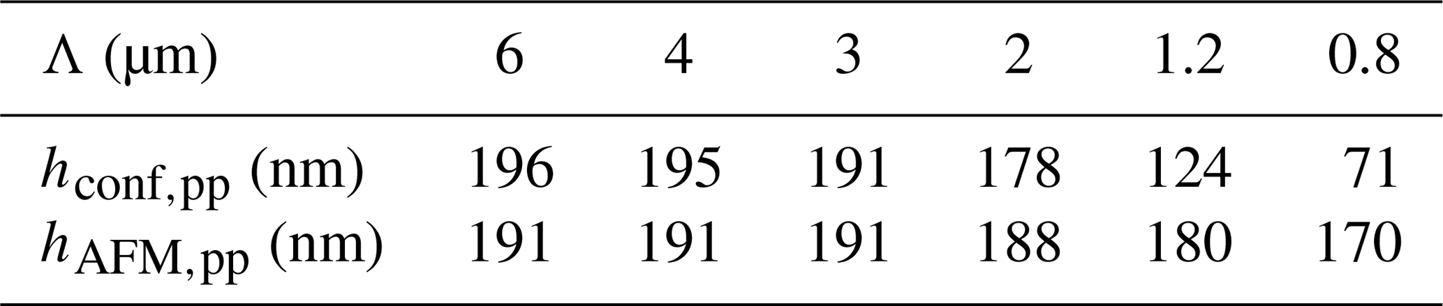
In order to obtain the ITF, various measurements are performed with the confocal microscope on a Simetrics RS-N standard, as presented in Table 2. This standard covers different rectangular gratings of various fundamental spatial frequencies Λ−1. The precision of the measured step height is increased by averaging 10 repeated measurement results for each spatial wavelength. As reference height, the measuring results of the AFM are used. The resulting ITF shows a decrease below a grating period of 3 µm, as displayed in Fig. 9c. From the course of the curve a wavelength Λ50 % of 925 nm is obtained, which is related to a decrease of 50 % of the real amplitude. As defined in DIN EN ISO (2517) and VDI/VDE (2655) for coherence scanning interferometry, Λ50 % equals twice the spatial wavelength ΛR pursuant to the Rayleigh criterion:
Based on the assumption that this relation is valid also for confocal microscopy, ΛR equals 462.5 nm. If χ equals 1, ΛR corresponds to the theoretical optical lateral resolution according to the Rayleigh criterion. However, here the empirical relation results in a multiplication with χ=1.45, which is a consequence of the deviation between the experimentally determined ΛR and the theoretical optical resolution.
Due to a comparison of the profile measured by the confocal microscope with a filtered AFM profile (according to Eq. 4), using various filter widths yields the best match for a sliding average with a width of 3ΛR as shown in Fig. 9d. Here, the ITF at 3ΛR corresponds to 0.75. Based on the results of the three different methods presented here to characterize the transfer behaviour of the confocal microscope, the latter method based on the experimentally determined ITF proved to be most suitable. This probably may be explained by optical aberrations of the confocal system due to imperfect optical components and maladjustment.
The multi-sensor measuring system makes it possible to conduct comparative measurements with various sensors at equal environmental conditions. In addition to the determination of the transfer characteristics of self-assembled sensors, the investigation of reference sensors is also possible. As a result of different working principles of the topography sensors used, artefacts or other deviations can be identified by comparative measurements. Since the measuring volume tracking is not fully implemented yet, the profiles shown in Fig. 6 are not measured on the exact same location on the specimen surface. For precise characterization of the transfer behaviour of a topography sensor, comparative measurements at equal locations are required. To reach this, further steps are essential. This includes the software implementation of all sensors in a common C ++ program and the proper calibration of the spatial deviations between the individual locations of the measurement fields of the sensors. In addition to positioning by the air bearing xy axes, the spatial conformity of the measurement fields can be increased by correlation of measured topographies. The desired maximum lateral deviation is 1 µm.
The accuracy of the height measurement of each reference sensor is characterized by different parameters for different instruments, namely the rms value for the AFM, the noise level for the confocal microscope and the residual value Rz0 for the stylus instrument. To ensure comparability, it is necessary to characterize both the individual reference sensors and the self-assembled topography sensors using the same parameter based on measurements on well-known surfaces.
As presented, the results of the AFM can be used as reference data for the characterization of other sensors. For a theoretical and numerical analysis of the measurement results of optical sensors, the results of the AFM can be used as input data to a simulation program introduced in Xie (2017), which is based on Kirchhoff theory and the Richards–Wolf model (Richards and Wolf, 1959).
Measurements at the same chirp structure using different topography sensors show the necessity of comparison measurements. Insight into the transfer behaviour of the sensors in the multi-sensor application is achieved by comparison of their chirp standard measurement results to those of the AFM. Therefore, the one-sided constrictions of the profiles measured by the optical sensors are explained by a sharp-combed structure instead of the originally assumed sinusoidal structure. Due to the sharp-combed structure the calculated nominal radius of curvature, based on the assumption of a sinusoidal structure, is too small. Thus the fine chirp profile is resolvable using the tactile stylus instrument with a tip radius of 2 µm. In spite of a lateral sampling interval of 500 nm the structure of the chirp standard is almost correctly measured. The presented comparative measurements between tactile and optical sensors indicate that depending on the surface structure of the measuring object, both techniques feature unique advantages, which are not available in a single-sensor system.
The multi-sensor measuring system is currently undergoing further development. As a final target, an automatic procedure for comparative measurements is intended as well as the continuous testing and improvement of the topography sensors.
The underlying measurement data are not publicly available and can be requested from the authors if required.
The authors declare that they have no conflict of interest.
This article is part of the special issue “Sensors and Measurement Systems 2018”. It is a result of the “Sensoren und Messsysteme 2018, 19. ITG-/GMA-Fachtagung”, Nürnberg, Germany, from 26 June 2018 to 27 June 2018.
The authors gratefully acknowledge the financial support of this project by
the DFG (Deutsche Forschungsgemeinschaft) under grant no. INST159/59-1 and
thank the company Mahr for providing the stylus instrument GD26.
Edited by: Rainer Tutsch
Reviewed by: two anonymous referees
Blu-ray Disc Association: White Paper Blu-ray Disc format: General, 5th Edition, available at: http://www.blu-raydisc.com, last access: 10 August 2018. a
Brand, U., Doering, L., Gao, S., Ahbe, T., Buetefisch, S., Li, Z., Felgner, A., Meess, R., Hiller, K., Peiner, E., Frank, T., and Halle, A.: Sensors and calibration standards for precise hardness and topography measurements in micro-and nanotechnology, in: Micro-Nano-Integration; 6. GMM-Workshop; Proceedings of, 1–5 pp., VDE, 2016. a
Corle, T. R. and Kino, G. S.: Confocal scanning optical microscopy and related imaging systems, Academic Press, 1996. a, b
Dabbs, T. and Glass, M.: Fiber-optic confocal microscope: FOCON, Appl. Optics, 31, 3030–3035, 1992. a
de Groot, P.: Principles of interference microscopy for the measurement of surface topography, Adv. Opt. Photonics, 7, 1–65, 2015. a
de Groot, P. and de Lega, X. C.: Interpreting interferometric height measurements using the instrument transfer function, in: Fringe 2005, 30–37 pp., Springer, 2006. a, b
de Groot, P., de Lega, X. C., Kramer, J., and Turzhitsky, M.: Determination of fringe order in white-light interference microscopy, Appl. Optics, 41, 4571–4578, 2002. a
DIN EN ISO 25178-604: Geometrical product specification (GPS) – Surface texture: Areal – Part 604: Nominal characteristics of non-contact (coherence scanning interferometry) instruments, 2013. a
DIN EN ISO 3274: Geometrical Product Specifications (GPS) – Surface texture: Profile method – Nominal characteristics of contact (stylus) Instruments, 1996. a, b, c
Doering, L., Brand, U., Bütefisch, S., Ahbe, T., Weimann, T., Peiner, E., and Frank, T.: High-speed microprobe for roughness measurements in high-aspect-ratio microstructures, Meas. Sci. Technol., 28, 034009, https://doi.org/10.1088/1361-6501/28/3/034009, 2017. a, b
Fewer, D., Hewlett, S., McCabe, E., and Hegarty, J.: Direct-view microscopy: experimental investigation of the dependence of the optical sectioning characteristics on pinhole-array configuration, J. Microsc., 187, 54–61, 1997. a
Fujii, A., Suzuki, H., and Yanagi, K.: Development of measurement standards for verifying functional performance of surface texture measuring instruments, J. Phys. Conf. Ser., IOP Publishing, 311, 012009, https://doi.org/10.1088/1742-6596/311/1/012009, 2011. a
Giusca, C. L. and Leach, R. K.: Calibration of the scales of areal surface topography measuring instruments: part 3. Resolution, Meas. Sci. Technol., 24, 105010, https://doi.org/10.1088/0957-0233/24/10/105010, 2013. a
Gu, M. and Sheppard, C.: Signal level of the fibre-optical confocal scanning microscope, J. Mod. Optic., 38, 1621–1630, 1991. a
Hagemeier, S. and Lehmann, P.: Multisensorisches Messsystem zur Untersuchung der Übertragungseigenschaften von Topographiesensoren (Multisensor measuring system for investigating the transfer characteristics of topography sensors), tm-Technisches Messen, 85, 380–394, 2018a. a, b
Hagemeier, S. and Lehmann, P.: Vergleichbarkeit des Übertragungsverhaltens optischer 3D-Sensoren an Kanten und Mikrostrukturen (Comparability of the transfer behavior of 3D optical sensors at edges and microstructures), 2. VDI-Fachtagung Multisensorik in der Fertigungsmesstechnik, VDI-Berichte Nr. 2326, 199–212, 2018b. a
Hagemeier, S., Tereschenko, S., and Lehmann, P.: High-speed laser interferometric distance sensor with reference mirror oscillating at ultrasonic frequencies, tm-Technisches Messen, https://doi.org/10.1515/teme-2019-0012, 2019. a
Harasaki, A. and Wyant, J. C.: Fringe modulation skewing effect in white-light vertical scanning interferometry, Appl. Optics, 39, 2101–2106, 2000. a
Jordan, H.-J., Wegner, M., and Tiziani, H.: Highly accurate non-contact characterization of engineering surfaces using confocal microscopy, Meas. Sci. Technol., 9, 1142, https://doi.org/10.1088/0957-0233/9/7/023, 1998. a
Kimura, S. and Wilson, T.: Confocal scanning optical microscope using single-mode fiber for signal detection, Appl. Optics, 30, 2143–2150, 1991. a
Kiselev, I., Kiselev, E. I., Drexel, M., and Hauptmannl, M.: Noise robustness of interferometric surface topography evaluation methods. Correlogram correlation, Surface Topography: Metrology and Properties, 5, 045008, https://doi.org/10.1088/2051-672x/aa9459, 2017. a
Kogelnik, H. and Li, T.: Laser beams and resonators, Appl. Optics, 5, 1550–1567, 1966. a
Krüger-Sehm, R., Bakucz, P., Jung, L., and Wilhelms, H.: Chirp-Kalibriernormale für Oberflächenmessgeräte (Chirp calibration standards for surface measuring instruments), tm-Technisches Messen, 74, 572–576, 2007. a
Lehmann, P., Tereschenko, S., and Xie, W.: Fundamental aspects of resolution and precision in vertical scanning white-light interferometry, Surface Topography: Metrology and Properties, 4, 024004, https://doi.org/10.1088/2051-672X/4/2/024004, 2016. a, b
Lehmann, P., Xie, W., Allendorf, B., and Tereschenko, S.: Coherence scanning and phase imaging optical interference microscopy at the lateral resolution limit, Opt. Express, 26, 7376–7389, 2018. a
Lin, S. K., Lin, I. C., and Tsai, D. P.: Characterization of nano recorded marks at different writing strategies on phase-change recording layer of optical disks, Opt. Express, 14, 4452–4458, 2006. a
Martínez-Corral, M.: Point spread function engineering in confocal scanning microscopy, SPIE Proceedings, 5182, 112–123, 2003. a
Mauch, F., Lyda, W., Gronle, M., and Osten, W.: Improved signal model for confocal sensors accounting for object depending artifacts, Opt. Express, 20, 19936–19945, 2012. a
Meinders, E. R., Mijiritskii, A. V., van Pieterson, L., and Wuttig, M.: Optical Data Storage: Phase-change media and recording, vol. 4, Springer Science & Business Media, 2006. a
Morrison, E.: The development of a prototype high-speed stylus profilometer and its application to rapid 3D surface measurement, Nanotechnology, 7, 37–42, https://doi.org/10.1088/0957-4484/7/1/005, 1996. a
Richards, B. and Wolf, E.: Electromagnetic diffraction in optical systems, II. Structure of the image field in an aplanatic system, Proc. R. Soc. Lond. A, 253, 358–379, 1959. a, b
Schake, M. and Lehmann, P.: Perturbation resistant RGB-interferometry with pulsed LED illumination, SPIE Proceedings, 10678, 1067805-01–1067805-12, https://doi.org/10.1117/12.2306221, 2018. a
Schake, M., Schulz, M., and Lehmann, P.: High-resolution fiber-coupled interferometric point sensor for micro-and nano-metrology, tm-Technisches Messen, 82, 367–376, 2015. a
Schulz, M. and Lehmann, P.: Measurement of distance changes using a fibre-coupled common-path interferometer with mechanical path length modulation, Meas. Sci. Technol., 24, 065202, https://doi.org/10.1088/0957-0233/24/6/065202, 2013. a
Schulz, M. and Lehmann, P.: Fasergekoppelter High-Speed-Sensor zum Messen optischer Funktionsflächen, 18. GMA/ITG-Fachtagung Sensoren und Messsysteme, 411–417, 2016. a, b
Seewig, J., Raid, I., Wiehr, C., and George, B. A.: Robust evaluation of intensity curves measured by confocal microscopies, SPIE Proceedings, 8788, 87880T, https://doi.org/10.1117/12.2020551, 2013. a
Seewig, J., Eifler, M., and Wiora, G.: Unambiguous evaluation of a chirp measurement standard, Surface Topography: Metrology and Properties, 2, 045003, https://doi.org/10.1088/2051-672X/2/4/045003, 2014. a
Sheppard, C. and Choudhury, A.: Image formation in the scanning microscope, Op. Acta, 24, 1051–1073, 1977. a, b, c
Tereschenko, S.: Digitale Analyse periodischer und transienter Messsignale anhand von Beispielen aus der optischen Präzisionsmesstechnik, Ph.D. thesis, University of Kassel, Germany, 2018. a
Tereschenko, S., Lehmann, P., Zellmer, L., and Brueckner-Foit, A.: Passive vibration compensation in scanning white-light interferometry, Appl. Optics, 55, 6172–6182, 2016. a
VDI/VDE 2655-1.3: Optical measurement of microtopography – Calibration of interference microscopes for form measurement, part 1.3, 2018. a
Weckenmann, A.: Koordinatenmesstechnik: flexible Strategien für funktions-und fertigungsgerechtes Prüfen, Hanser, 2012. a
Wiedenhöfer, T.: Multisensor-Koordinatenmesstechnik zur Erfassung dimensioneller Messgrößen, tm-Technisches Messen, 78, 150–155, 2011. a
Wilson, T.: Confocal microscopy, Academic Press London, 1990. a
Xiao, G., Corle, T. R., and Kino, G.: Real-time confocal scanning optical microscope, Appl. Phys. Lett., 53, 716–718, 1988. a
Xie, W.: Transfer Characteristics of White Light Interferometers and Confocal Microscopes, Ph.D. thesis, University of Kassel, Germany, 2017. a, b, c
Xie, W., Hagemeier, S., Woidt, C., Hillmer, H., and Lehmann, P.: Influences of edges and steep slopes in 3d interference and confocal microscopy, SPIE Proceedings, 9890, 98900X, https://doi.org/10.1117/12.2228307 2016. a
Xie, W., Hagemeier, S., Bischoff, J., Mastylo, R., Manske, E., and Lehmann, P.: Transfer characteristics of optical profilers with respect to rectangular edge and step height measurement, SPIE Proceedings, 10329, 1032916, https://doi.org/10.1117/12.2270185, 2017. a, b