3.1 Coordinate transformations

One key feature of SimOptDevice is its easy way to transform coordinates from any local system to any other coordinate system within the defined structure (see Fig. 1). Coordinates are defined as homogeneous coordinates (see e.g. Cox et al., 2007, p. 357 ff.). Rotations and translations can be represented as matrices, and it is simple to connect transformations and compute a transformation's inverse. Homogeneous coordinates for describing points in ℝ³ have four components. A vector v=(x, y, z)^T is represented in homogeneous coordinates as ${\mathit{v}}^{\prime }=(x^{\prime }$, $y^{\prime }{z}^{\prime }$, w)^T, where w≠0 is arbitrary and $x^{\prime }=x/w$, $y^{\prime }=y/w$, and $z^{\prime }=z/w$. Usually, w is set to one.

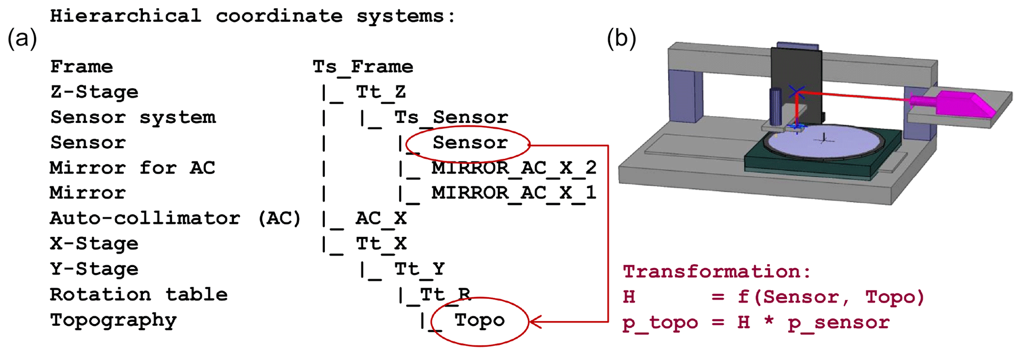
Figure 1Example of the hierarchical structure of coordinate systems in SimOptDevice. (a) The plot of a coordinate system tree example is shown. The left column lists the element names; the right column shows a sketch of the hierarchical structure of the coordinate systems. (b) The corresponding instrument is illustrated. The position and orientation of each of the instrument's subsystems are defined with respect to the superordinate system through a transformation of homogeneous coordinates. A transformation matrix H can be computed for transformations from one system to another (see Eq. 2). It is a function of the source system and the destination system (in this example Sensor and Topo, respectively). The common superordinate system Ts_Frame is needed for the computation of the transformation matrix (cf. Eq. 2). Subsequently, coordinates of a point in one system can be transformed to any other system by multiplication by the corresponding transformation matrix H.

Download

With this coordinate definition, a translation or rotation is represented by a 4×4 matrix:

Rotations about the other axes are defined analogously. The composition of several homogeneous transformations H₁, H₂, …, H_N is equal to a single homogeneous transformation

Using Eq. (1), the translation and rotation of a coordinate system with respect to its superordinate system are represented by a single matrix. The inverse of a homogeneous transformation is represented by the inverse of the corresponding transformation matrix. The aforementioned transformation from one local source system S_a to another destination system S_b is performed with the help of a common superordinate system S_c:

For a more comprehensive introduction to homogeneous coordinates, see e.g. Cox et al. (2007) or Hartley and Zisserman (2003).

3.2 Ray tracing

Ray propagation through the defined object is performed by sequential ray tracing. For this tracing method the order of elements passed by a ray is known in advance and optical paths are computed element by element. SimOptDevice computes the ray paths locally in each optical element system. At the boundary T_i between two elements (e.g. a surface of a lens), the current intersection point p_i of the ray with that boundary along with the new ray direction e_i are calculated in the new local system (cf. Sect. 3.1). The ray is then traced until it intersects with the next boundary, and so on. The intersection point with T_i and the new direction are a function of the previous intersection point and ray direction:

Function f_i entails performing the following steps (cf. Fig. 2 for an illustration):

1. transformation of p_i−1 and e_i−1 from system T_i−1 to T_i,

2. calculation of the ray's geometrical path length l_i between T_i−1 and T_i,

3. determination of next intersection point ${\mathit{p}}_i={\mathit{p}}_{i-\mathrm{1}}+l_i\cdot {\mathit{e}}_{i-\mathrm{1}}$,

4. calculation of normal vector n_i on T_i in p_i, and

5. calculation of the new ray direction e_i according to the laws of refraction and reflection.

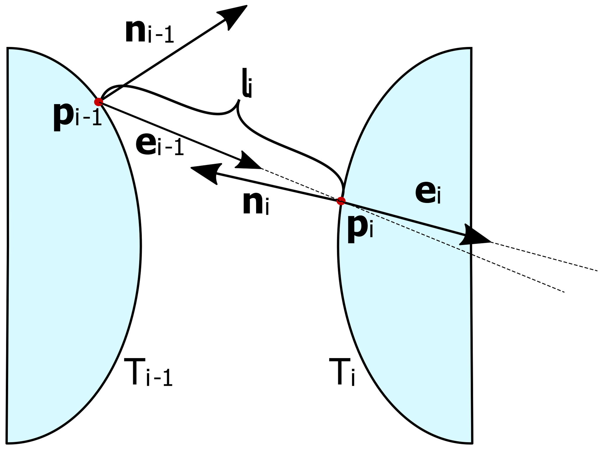
Figure 2Schematics of a ray tracing step. Each topography T has its own coordinate system. The intersection point p_i with topography T_i is computed from the previous intersection point p_i−1 and the previous ray direction e_i−1. Subsequently, the new ray direction e_i at T_i is computed according to the laws of reflection and refraction.

Download

This is classical ray tracing with the particular feature that at each boundary the intersection point and the new direction are calculated in the new local coordinate system. Step 3 is calculated analytically for planes and spherical surfaces and has to be calculated numerically for more complex surfaces like Zernike surfaces, aspheres, or surfaces described by a Gauss function. If the ray passes N surfaces, there are N different functions f_i. The last intersection point and ray direction can be expressed as a function of the start point and direction by concatenation of functions f₁ to f_N:

Furthermore, for each crossing of a boundary T_i a Jacobian matrix containing the partial derivatives of the intersection point p_i and the ray direction e_i with respect to the previous intersection point p_i−1 and the previous ray direction e_i−1 is calculated. It is associated with Eq. (3) and has the following form:

where x_i and y_i are the x and y components of the point p_i, and ${\widehat{x}}_i$ and ${\widehat{y}}_i$ are the x and y components of the direction e_i. We only need the derivatives with respect to the x and y components, since the intersected topographies are known and the z component is fixed at the intersection point. Since the direction vector has unit length, its z component can be calculated by $\widehat{z}=\sqrt{\mathrm{1}-{\widehat{x}}^{\mathrm{2}}-{\widehat{y}}^{\mathrm{2}}}$. The Jacobian matrix J corresponding to the concatenation of N−1 interfaces i=1 … N−1 associated with Eq. (4) is obtained by multiplication of the corresponding matrices:

The inverse Jacobian matrix J⁻¹ describes partial derivatives of the ray's behaviour along the same path in the opposite direction. These Jacobian matrices are used extensively when performing the ray aiming. Their usage is explained in more detail in Sect. 3.3. A detailed description of the ray tracing and ray aiming procedures can also be found in Fortmeier (2016, in German).

3.3 Ray aiming

Given a start point p₀ and an end point ${\mathit{p}}_N^{\mathrm{dest}}$ the task of ray aiming is to find the start direction e₀ from p₀ in order to minimize the distance between p_N and the desired end point ${\mathit{p}}_N^{\mathrm{dest}}$ (see Fig. 3):

where $\left|\right|\cdot \left|\right|$ denotes the Euclidean norm and p_N is reached through application of ray tracing for a chosen start direction e₀. For successful ray aiming the resulting norm in Eq. (6) is close to zero. This is usually a highly nonlinear problem. It can be solved using one of MATLAB^®'s parallel nonlinear solver routines, e.g. lsqnonlin. The latter is a solver for nonlinear least-squares problems in which the trust-region-reflective or Levenberg–Marquard algorithm can be applied. For better convergence of the solver, the ray tracing Jacobian matrix from Eq. (5) is utilized in this step. The Jacobian matrices calculated during ray tracing are used to update the start direction e₀ when minimizing the distance between point p_N and point ${\mathit{p}}_N^{\mathrm{dest}}$. Furthermore, SimOptDevice delivers the Jacobian matrices for the change in total optical path lengths with respect to changes in a point p_i or a ray direction e_i for each surface T_i (Fortmeier et al., 2014). It is calculated analytically, thereby omitting the computationally expensive extra ray tracing steps for the numerical differentiation. The Jacobian matrices for ray aiming are important in many interferometric applications, e.g. the tilted-wave interferometer (cf. Sect. 4), where the change in the optical path length of a ray is a significant quantity of the experiment.

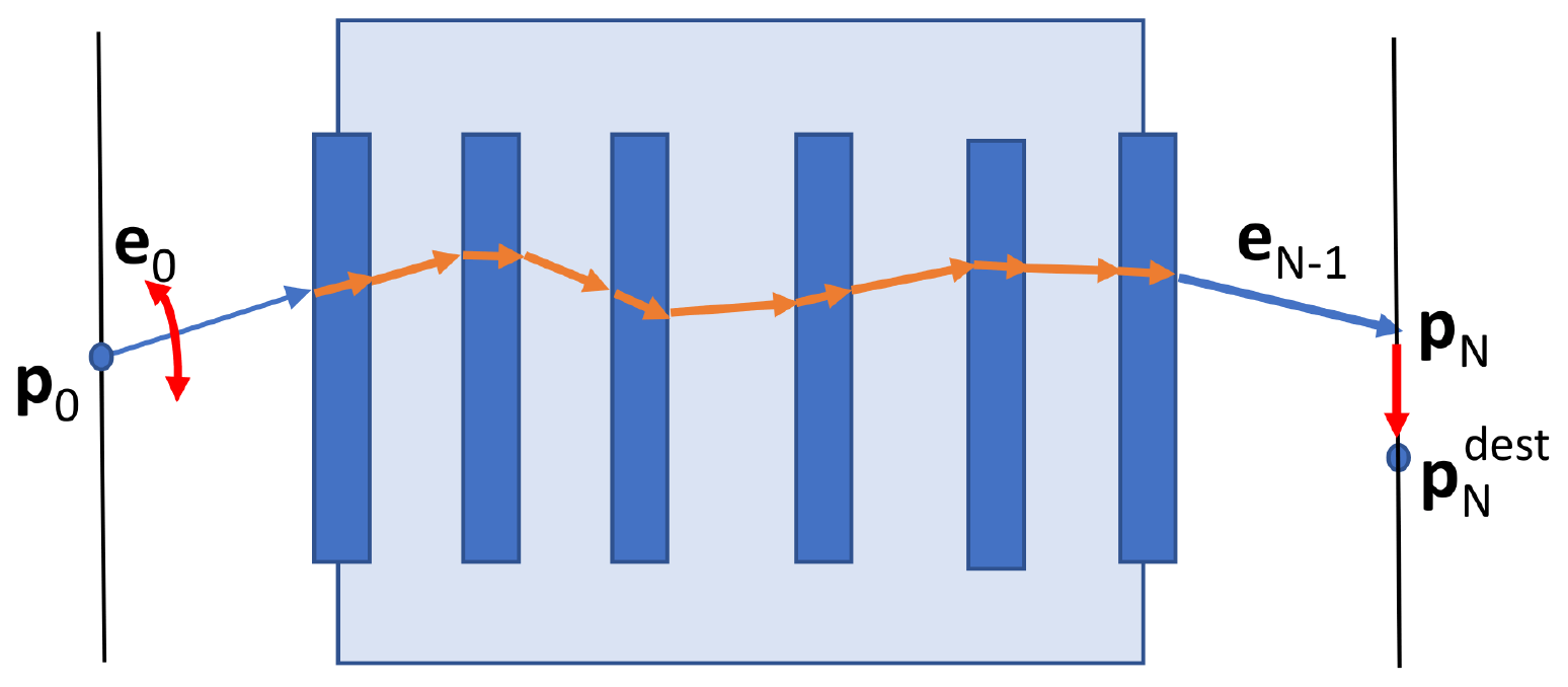
Figure 3Ray aiming principle: the start and end points p₀ and ${\mathit{p}}_N^{\mathrm{dest}}$ of a ray are given. The task is to find the correct start angle e₀ such that the desired end point is hit. This is achieved by minimizing the distance between points p_N and ${\mathit{p}}_N^{\mathrm{dest}}$, when p_N is reached through application of ray tracing for a chosen start direction, e₀.

Download

A requirement for successful ray aiming is that the destination point ${\mathit{p}}_N^{\mathrm{dest}}$ can be reached. Therefore, the valid area on the CCD (or any other final surface) is determined in a preceding step. A ray aiming between the light source and some characteristic points at the smallest aperture in the optical system is performed. The final ray directions at the aperture are used to trace the rays to the CCD, thereby defining the area that can be reached by rays from the sources. A ray aiming is regarded as successful if the norm of the difference in Eq. (6) is smaller than 1 nm. Local minima that prevent the algorithm from converging are detected and such rays are masked. Using the Jacobian matrix, the ray aiming usually converges in about four steps. Without the Jacobian matrix this takes approximately 12 to 15 steps, depending on the particular situation.

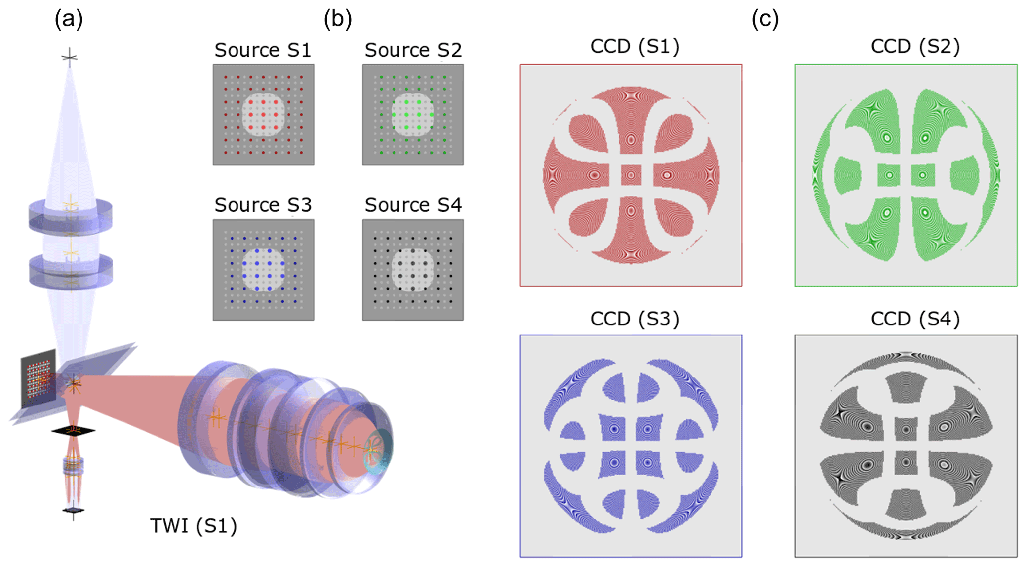
Figure 4Examples from the tilted-wave interferometer (TWI) simulation. (a) Ray paths through the instrument. Source array, reference and test arms, and detector (CCD). (b) The sources of the laser array are switched on in four groups (S1 to S4); (c) simulated interferograms on the CCD for each of the source groups for an asphere example.

Download