the Creative Commons Attribution 4.0 License.
the Creative Commons Attribution 4.0 License.
 | 20 Sep 2018
DAV3E – a MATLAB toolbox for multivariate sensor data evaluation
Manuel Bastuck
Tobias Baur
Andreas Schütze
We present DAV3E, a MATLAB toolbox for feature extraction from, and evaluation of, cyclic sensor data. These kind of data arise from many real-world applications like gas sensors in temperature cycled operation or condition monitoring of hydraulic machines. DAV3E enables interactive shape-describing feature extraction from such datasets, which is lacking in current machine learning tools, with subsequent methods to build validated statistical models for the prediction of unknown data. It also provides more sophisticated methods like model hierarchies, exhaustive parameter search, and automatic data fusion, which can all be accessed in the same graphical user interface for a streamlined and efficient workflow, or via command line for more advanced users. New features and visualization methods can be added with minimal MATLAB knowledge through the plug-in system. We describe ideas and concepts implemented in the software, as well as the currently existing modules, and demonstrate its capabilities for one synthetic and two real datasets. An executable version of DAV3E can be found at http://www.lmt.uni-saarland.de/dave (last access: 14 September 2018). The source code is available on request.
- Article
(7220 KB) -
Supplement
(151 KB) - BibTeX
- EndNote


In recent years, a new paradigm has been developing in science, introducing a whole new field of both research and tools: big data (Chang et al., 2014; Kitchin, 2014). With enough data and computing power, a wide variety of systems, previously inaccessible to physical models due to their complexity, have become available to scientific description and treatment with the use of statistical models. New challenges arise for data processing because (semi-)automatic approaches and smart assistant systems are essential to handle and evaluate the huge amounts of data.
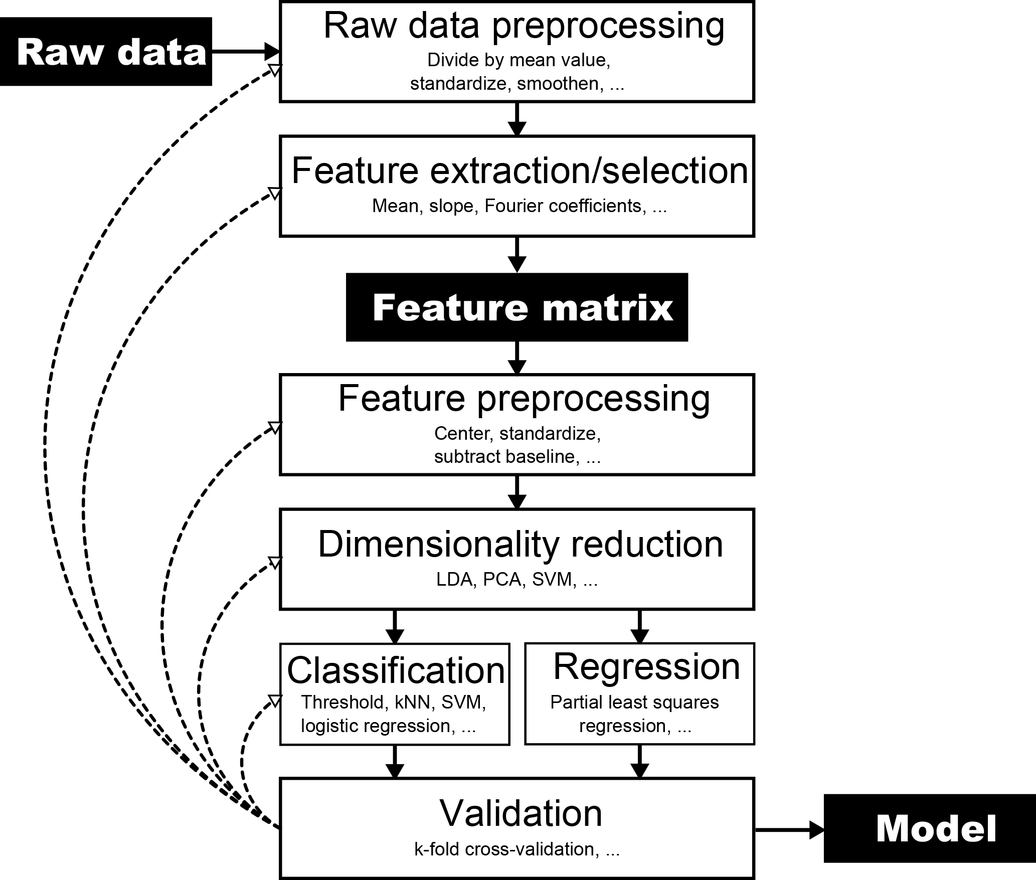
Figure 1Flowchart of the steps involved in building a statistical model from raw data. The validation step is crucial to check the model's performance. Any step and its parameters in the process influence the model performance. However, the exact way is usually hard to predict, which results in a time-consuming trial-and-error process to find a model that performs well. Most available software packages for machine learning or statistical model building usually start at the feature matrix, thus ignoring the need for feature extraction from the raw data, which is a crucial step, especially, but not only, for cyclic sensor signals.
Many software packages exist for statistical data evaluation or machine learning. A non-exhaustive list includes commercial and closed-source packages like SPSS Statistics (IBM), Minitab (Minitab Inc.), Statistica (StatSoft), and RapidMiner (RapidMiner, Inc.), as well as open-source alternatives like Weka (University of Waikato), R (The R Foundation), and orange (University of Ljubljana). The PLS_Toolbox (Eigenvector Research, Inc.) is a noteworthy member of this list by being commercial, but partly open-source, and the only of the tools known to the authors that is MATLAB-based. Many of these programs can be extended by the user with modules written in Python or Java, so, in general, it is often possible to add missing features and functions oneself. However, mechanical or electronic engineers, who most often work with sensors and sensor systems, often do not have any, or little, training in programming and data science in general. The existing software packages usually try to be as flexible as possible, which can seem overwhelming to new users. From personal experience, we know that many engineers in this field prefer MATLAB over Java or Python due to its out-of-the-box numerical abilities while providing a simple and easy-to-learn script language.
However, this observation was not the only reason for the development of DAV3E (Data Analysis and Verification/Visualization/Validation Environment). A problem common in many statistical software packages, including, to the best of the authors' knowledge, the PLS_Toolbox, is the assumption that the data are already available in the form of a feature matrix (Fig. 1). This assumption does not take into account that features must often first be generated, or extracted, from raw data, which is a highly relevant and all too often neglected part of the evaluation process.
A prime example of this issue is the cyclic operation of sensors. An operation mode called temperature cycled operation (TCO) has long been known (Eicker, 1977; Lee and Reedy, 1999) to improve sensitivity and selectivity for chemical sensors and gas sensors in particular (Bur, 2015; Reimann and Schütze, 2014). TCO works by collecting data from the sensor at different operating temperatures. The operating temperature influences the physical and chemical reactions on the sensor surface and, thus, the sensor behavior. The result is an array of sensor responses very similar to an actual sensor array, which is why this approach is also known as a virtual multisensor system (Reimann and Schütze, 2014; Schütze et al., 2004). In this example, one temperature cycle can take several minutes, which is the effective sampling period of the sensor. However, the sensor must actually be sampled much faster, usually in the range from Hz to kHz, during the cycle. The information about the present gas is not contained so much in one of the resulting several thousand points in one cycle, but rather in the overall signal shape during one cycle. To avoid the curse of dimensionality (Böhm et al., 2001; Gutierrez-Osuna, 2002; James et al., 2013), it is therefore necessary to extract information-rich features from the cyclic sensor signal.
Several other approaches following the same principle exist, e.g., voltammetry in electronic tongues (Apetrei et al., 2004), gate bias cycled operation (GBCO) (Bur, 2015) for gas-sensitive field-effect transistors (GasFETs) (Andersson et al., 2013), or exploitation of the working cycle of hydraulic machines for online condition monitoring of those machines (Helwig et al., 2015).
Several methods have been established for feature extraction from cyclic signals. TCO-MOX sensor signals are often processed by a fast Fourier transform (FFT) (Heilig et al., 1997) or a discrete wavelet transform (DWT) (Cetó et al., 2014; Ding et al., 2005; Huang et al., 2006; Moreno-Barón et al., 2006), usually in combination with a suitable, i.e., sine wave, temperature cycle. Other approaches include windowed time slicing (Apetrei et al., 2007; Gutierrez-Osuna and Nagle, 1999) or principal component analysis (PCA) (Winquist et al., 1997). A comprehensive review of these and more methods is given in Sect. II A1 in Marco and Gutierrez-Galvez (2012). In contrast to these projection methods, DAV3E specializes in extracting shape-describing features from a cyclic signal. It has been shown that such features can outperform FFT and DWT features (Gramm and Schütze, 2003). They are also very easy to compute, unlike DWT or other complex decompositions, so they can easily be implemented in cheap hardware, i.e., microprocessors. Finally, the feature extraction implementation in DAV3E is a superset of the above-mentioned methods: if desired, DWT can still be applied to the whole cycle, but if a physical model suggests that, e.g., the slope in one specific part of the cycle is a suitable feature (Baur et al., 2015), this slope can additionally be extracted to improve the model. To the best of the authors' knowledge, there is no software which provides both aspects of statistical data evaluation, i.e., shape-describing feature extraction and statistical model building. In particular, a tool for manual, graphical feature extraction from cycles was not available before. But implementing only this functionality could easily lead to inefficient workflows since the user would constantly have to switch between at least two different software tools.
As a solution to this problem, we have developed DAV3E, a MATLAB-based, object-oriented framework. It covers the cycle-based data preprocessing and feature extraction missing in contemporary data-mining software packages and sensor-aware functions like correction of time offset and sample rate without resampling, as well as simple or hierarchical statistical models, both for classification and regression. The graphical user interface (GUI) leads the user through the process and, thus, is suitable for beginners and advanced users, which is especially important in fields in which new people are constantly starting their work on statistical data evaluation, like universities. For advanced users who prefer a textual interface or want to perform batch processing or other kinds of automation, the functionality is also available via the command line. To further aid the user, the evaluation is supported by static, animated, or interactive visualizations in every step.
2.1 Workflow
The model-building workflow implemented in DAV3E is depicted in Fig. 1 and follows the process outlined by Gutierrez-Osuna for machine olfaction in (Gutierrez-Osuna, 2002). Raw data are the data collected from sensors or lab equipment. The data are assumed to be of a cyclic nature; i.e., there is at least one setpoint parameter which repeats a cyclic pattern over time. Hence, each data stream can also be seen as a matrix with as many rows as there are cycles in the whole measurement, and as many columns as there are data points in one cycle. The typical length of a cycle is in the order of seconds or minutes, with sampling rates in the order of Hz or kHz. However, the exact values can vary greatly between use cases. Note that this approach also covers simple time series data, if not only a single value but a certain time window is used for evaluation.
The cyclic approach offers some unique preprocessing methods for the raw data, e.g., dividing each cycle by its mean value to mitigate sensor drift (Gramm and Schütze, 2003). At the same time, the information contained in the cycles mean value is then eliminated. Whether drift compensation or more information is more important for the model performance is often not immediately clear and must be determined by validating the final model. This is just one of many parameters influencing the model, and often model validation and subsequent adjustments to the parameters, i.e., trial and error, is the only way to improve model performance as there is no guarantee that a certain data evaluation algorithm will yield optimum results.
Another special feature of cyclic sensor operation is the way features are extracted from the raw data. One cycle can have many thousands of highly correlated data points or features. Both the high number (Hastie et al., 2009; James et al., 2013) as well as the collinearity (Næs and Mevik, 2001) can cause problems like instabilities in many machine learning methods, so the dimensionality of the feature space must be reduced. This reduction is achieved by describing the shape of the signal with as few parameters as possible while maintaining most of the information. For example, an area in the cycle where the signal is nearly flat over thousands of points is described equally well with just one parameter: the mean of all of these points. This step typically reduces the number of features by 90 % or more and results in less correlation between the features. Which parts in the cycle and which fit functions are used is often determined manually, so the result can depend on the experience of the user. In rare cases, a rough physical model allows for a more targeted extraction of features from the raw data. In all cases, the result of this step is a feature matrix with the same number of rows (observations) as the raw data, but fewer columns (features). Most machine learning tools assume the data to have this or an equivalent shape.
Hence, the following steps are the steps involved in every multivariate statistical analysis (Gutierrez-Osuna, 2002). The feature columns can be preprocessed, e.g., standardized, to remove scaling and achieve more stable numerical results (van den Berg et al., 2006). The same can be done to the target vectors, if they are numeric, e.g., to linearize a logarithmic sensor response. Further dimensionality reduction is often done using unsupervised principal component analysis (PCA) (Gutierrez-Osuna, 2002; Risvik, 2007) or supervised linear discriminant analysis (LDA) (Gutierrez-Osuna, 2002). Both steps are optional, and dimensionality reduction is often a part of classification or regression (“prediction” in general), as in the case of support vector machines (SVMs) (Smola and Schölkopf, 2004) or partial least squares regression (PLSR) (Abdi, 2010; Geladi and Kowalski, 1986). Other classifiers available in DAV3E are k nearest neighbors (kNN) (Hastie et al., 2009), discriminant analysis (DA) (Hastie et al., 2009), logistic regression (LR) (Hastie et al., 2009), and more. It is necessary to validate the whole evaluation chain to prevent overfitting, an effect whereby a model fits the training data very well, but is not able to predict new data correctly (Hawkins, 2004). Validation can be done with new data when the correct outcomes are known for each observation. If such a validation dataset is not available, validation is still possible, e.g., with k-fold cross-validation (Browne, 2000; Kohavi, 1995), which uses one part of the dataset for training and the other for testing. The eventual performance of the model is then determined with a test dataset which contains only data that were never used in training or validating the model.
2.2 Data structure and fusion
DAV3E saves imported data in a hierarchical structure consisting of measurement, cluster, and sensor objects. A sensor is the smallest unit and contains the data associated with the sensor. This can be data from an actual physical sensor, e.g., an acceleration or gas sensor, one of many channels of a scientific instrument, e.g., the measured voltage of channel 1 of a multichannel data acquisition system, or a virtual sensor which is computed from other physical sensors, e.g., the resistance which is computed as the quotient of voltage and current. Each sensor can be assigned a unique data evaluation chain with different raw data preprocessing and feature extraction algorithms, which accounts for the fact that data from different sensors can be very dissimilar.
Sensors are organized in clusters, which contain information about time offset (to a reference time) of the data acquisition, sampling rate, and number of data points per cycle. While this information could well also be saved directly with each sensor, there are often natural “groups” of sensors in real measurements, e.g., three channels from a device that measures (1) voltage and (2) current over (3) time. Two virtual sensors, “virtual data points” and “virtual time”, are derived from each cluster's sampling rate and offset information. They serve as default abscissa for sensors in this cluster for plots or during feature extraction. Default values are useful because, quite often, information about time and/or data points is not provided as a sensor. As virtual sensors are computed dynamically, later changes to time offset or sampling rate are as easy as changing the specific value, and the time information is automatically adapted accordingly.
Clusters are contained in measurements. A measurement always has a defined starting time and date and can thus provide a time reference for its clusters. It also stores time ranges during which the environmental conditions influencing the sensors, i.e., gas concentrations or system failure states, were constant. This is only useful if not all points in time of the measurement are of interest for the evaluation, which is, however, often the case. Experimental systems are often proprietary and not integrated with each other. This means that, for example, the gas sensor data acquisition and the test environment, e.g., a gas mixing apparatus (Helwig et al., 2014) providing defined gas mixtures for the characterization, run in parallel, but are not necessarily exactly synchronized. It is thus easier to start both systems and combine their data afterwards, which will result in undefined states when the gas mixing apparatus is changing states while the sensor proceeds with its current cycle. This and potentially a few following cycles are obtained under unknown conditions and must therefore be excluded from the evaluation. In a measurement, relevant time segments with known environmental conditions can be selected (or imported) so that only cycles recorded during these times are considered for further evaluation.
All sensors in the same measurement will add to the number of features available in the observations in this measurement; i.e., the sensors are fused in parallel. Consequently, the environmental conditions defined in the measurement are automatically assumed by newly added sensors without any action from the user. Sensors in different measurements, however, are added in series; i.e., they add to the total number of observations. Sensors from different measurements are associated by their name, so data from identical sensors are automatically combined (Fig. 2).
2.3 Programming concepts and plug-ins
One focus during the development was easy extendibility of all important aspects of the software. The object-oriented design helps to keep a clear structure and maintainable code. Additionally, a plug-in concept was implemented that allows all users with basic MATLAB knowledge to add new functions. Contrary to other programming languages, MATLAB knowledge is widespread amongst engineers, who are the main target users of DAV3E. If necessary, scripts in other languages like R or Python can easily be accessed from within MATLAB. Currently, the plug-in system covers the following algorithm types: dimensionality reduction, feature extraction, feature and response preprocessing, data import sources, virtual sensor computation, raw data preprocessing, postprocessing, classifiers, regressors, and validation. A subset of those, i.e., dimensionality reduction, classifiers, and regressors, provides the addition of custom plots as plug-ins.
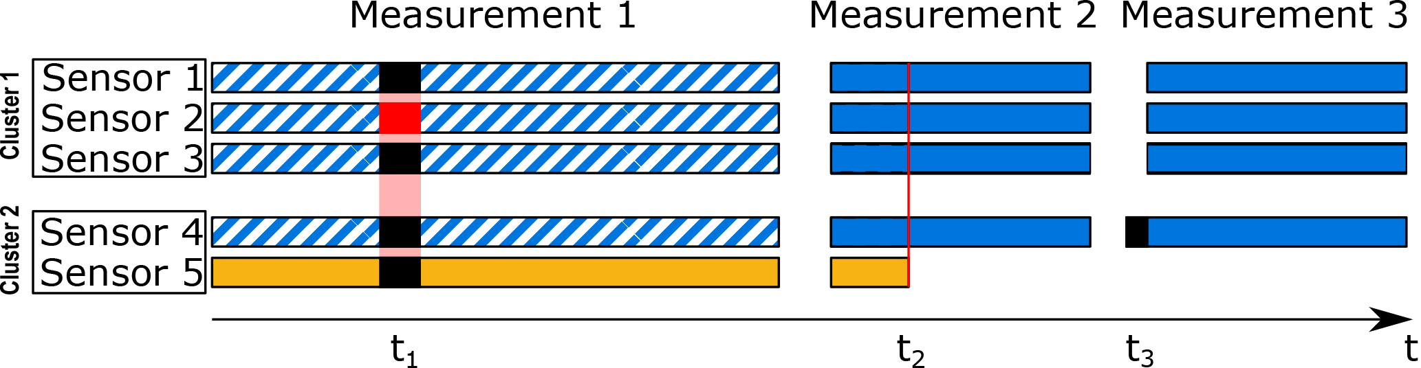
Figure 2Illustration of data fusion with five sensors from two different sources (cluster 1/2). If one sensor sends faulty or noisy data over some time (sensor 2 at t1), DAV3E will automatically ignore all data during that time in the fused dataset. If a sensor fails (sensor 5 at t2), the user can choose to have more observations, but without that sensor (blue data), or to include all sensors, but with fewer observations (orange data). If a sensor starts too early (sensor 4 at t3), its data will be ignored until data from all sensors are available. Such events can either be annotated by the user or imported directly from the test setup if the data are available.
For each type of plug-in, a template file defines available functions with a fixed interface, so all available data can easily be accessed and the user can concentrate on the correct implementation of their function instead of programmatic technicalities.
Depending on the sample rate and duration of the measurement, the sensor dataset can become rather large. Several gigabytes are easily reached, and certain applications in condition monitoring have already produced data with several tens of terabytes. Currently, DAV3E's ability to handle such data are still limited by the size of system memory (RAM, random access memory). However, measures have been taken not to use up more space than necessary.
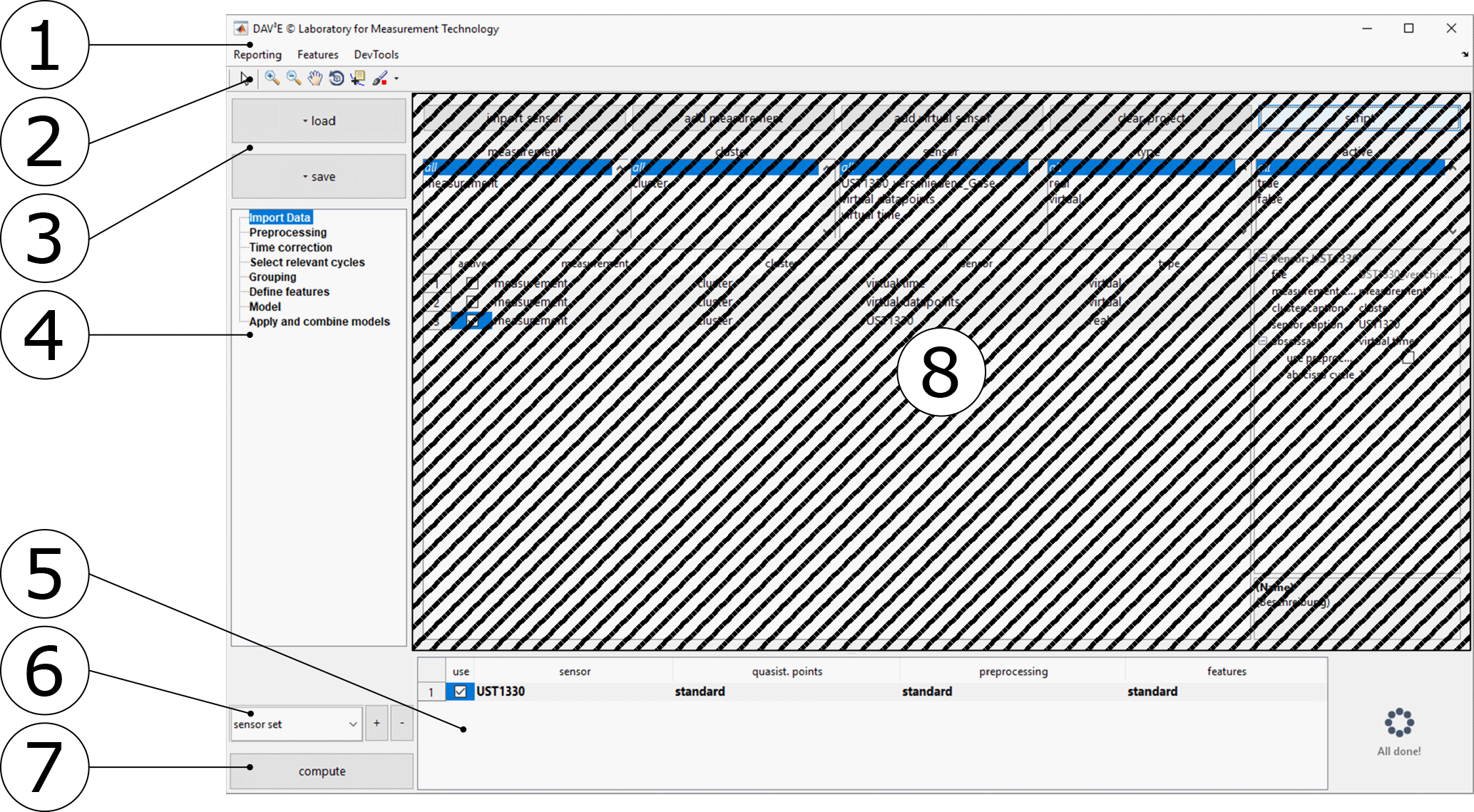
Figure 3Main GUI with menu bar (1), toolbar (2), load and save buttons (3), the list of modules (4), the list of selected sensors (5), the current sensor set (6), the compute button for features (7), and the currently selected module (8, shaded).
One important aspect is to omit resampling of the data. Downsampling can lead to loss of information, while upsampling can lead to significantly increased size in memory, especially if the dataset contains one or more sensors with very high sample rates. In the evaluation process, selections must be made in the data which, ultimately, must refer to the same point in time for all sensors in a measurement to ensure consistent results for sensors with different offsets, sample rates, or cycle lengths. Any selection is thus stored as a timestamp. Given an arbitrary sensor, this timestamp can be used to calculate which point or part of its data should be selected.
2.4 Dependencies
The toolbox is designed to have as few dependencies on other MATLAB toolboxes as possible. Most dimensionality reduction, classification, and regression methods rely on their implementation in the Statistics and Machine Learning Toolbox. The LDA projection can be computed by manova1 from this toolbox. In a newer version of DAV3E currently in development, however, we replace most of these functions by our own implementations. These are based on the MATLAB implementation, but drop many type checks, etc., resulting in quicker execution. Checking the input to these low-level functions is not necessary in this context as errors are already caught by higher level functions.
The report functionality additionally needs the Report Generator, and special, but nonessential functions rely on the Curve Fitting Toolbox (fitting Gauss peaks) and the Econometrics Toolbox (feature correlation plot, corrplot). Especially the latter could easily be rewritten, if necessary. The same applies to the function that is used to determine well-distinguishable colors for new elements which, coming from FileExchange, makes uses of the Image Processing Toolbox. This functionality can easily be bypassed if the toolbox is not available.
DAV3E is compatible with MATLAB R2016b or later.
2.5 Graphical user interface
A graphical user interface (GUI) is the main way the average user actively interacts with a computer program. It gives a graphical representation of all options the user currently has which can lead to a more efficient workflow. Without a GUI, the user can call functions of the program directly in the command line, which can be of benefit to more advanced users when performing complex tasks or some degree of automation. Both interfaces are available in DAV3E; however, as statistical methods tend to have many different options to tune their behavior, it is often easier to see a list of available options in a GUI instead of memorizing or researching different parameters. Additionally, research often needs to explore its datasets looking for distinct features, a task for which static, animated, or interactive plots, an essential part of the GUI, are very helpful. For an example of the command line interface, refer to the supplement.
The GUI is based on the GUI Layout Toolbox (Tordoff and Sampson, 2014), which enables layout-based GUI programming in MATLAB. MATLAB GUIs are based on Java and the JIDE framework (jidesoft). Not all the framework's elements and functionality are currently implemented, but can relatively easily be added directly or retrofitted with the findjobj function (Altman, 2012). For DAV3E, the standard MATLAB GUI components have been extended with PropertyTables, JTrees, and JTables.
The main GUI (Fig. 3) consists of a frame providing a menu bar (1), toolbar (2), load and save buttons (3), a list of all loaded modules (4), a table showing the currently active sensors (5), a drop-down menu to select the current sensor set (6), and a button to compute features from the current configuration (7). GUI modules (8) can communicate with the main GUI via defined interfaces and are otherwise decoupled from the main GUI and each other. A module can be added with a plug-in system similar to the one described before, and performs one or more specific functions by reading or manipulating the data in the underlying structure of measurements, clusters, and sensors.
In Sects. 4 and 5, various modules and features of DAV3E are shown for three example datasets to facilitate easier understanding of the descriptions. The datasets were chosen from different areas to demonstrate why a high versatility of the toolbox is required.
3.1 Hill-Valley dataset
This dataset is publicly available (Graham and Oppacher, 2018) from the UCI machine learning repository (Lichman, 2013). It consists of a training set with 606 observations, i.e., cycles, with 100 data points each, and a test set with the same dimensions. The data in each cycle show either a hill or a valley when plotted, and the classification task is to discriminate hill cycles from valley cycles. The dataset is provided both with and without noise. For this demonstration, only the noisy variant is used. Before the data are imported into DAV3E it is first sorted by the class information, which allows easier handling afterwards.
3.2 Gas sensor dataset
In the gas sensor dataset (Bastuck and Fricke, 2018), the commercial gas sensor GGS1330 by UST (UmweltSensorTechnik GmbH, Germany) was exposed to different concentrations of different gases in synthetic air at constant relative humidity: carbon monoxide, CO (100, 200, 300 ppm), ammonia, NH3 (75, 150, 225 ppm), nitrogen dioxide, NO2 (10, 20, 30 ppm), and methane, CH4 (500, 1000, 1500 ppm). It was operated with a triangle-shaped TCO cycle, rising linearly from 200 to 400 ∘C in 20 s, and decreasing back to 200 ∘C in another 20 s. Each gas exposure lasted for 15 min and contained at least 20 complete sensor temperature cycles, with a total of 190 observations.
3.3 Condition monitoring dataset
The condition monitoring dataset (Helwig et al., 2018) is taken from Helwig et al. (2015), where more detailed information can be found. Several sensors for monitoring pressure, vibration, electrical power, and other variables have been recorded from a hydraulic machine with a 1 min working cycle. Some sensors were sampled with 1 Hz, some with 10 Hz, and some with 100 Hz, resulting in approx. 50 000 sensor values per cycle. Faults with different grades of severity like leaks, valve malfunction, and others in all possible permutations were then simulated in the system. The aim is to classify the type of fault and quantify its severity. The total number of observations is 1260.
4.1 Data import
The first step in the evaluation process is to import experimental data. The button “import sensor” opens a Choose File dialog in which all data types that DAV3E can handle can be selected. Import routines are currently implemented for files with simple structures like CSV or MAT, as well as for more complex, proprietary formats stored as HDF5 (HDF5 Group, 2016), for instance. The expected format is always a data matrix in which each row corresponds to one cycle, i.e., observation. The columns consequently represent the sampling points, i.e., features. The import plug-in system provides an easy means of adding data types or even import from databases.
Importing the first sensor automatically creates a new measurement. When a second sensor is to be imported, it can either be added in parallel to an already existing sensor, i.e., in the same measurement, or to a new measurement, i.e., in series. Parallel sensors add features, and serial sensors add observations to the dataset. To keep a good overview, especially with many sensors, the table can be filtered by measurement, cluster, sensor, type, and selection, with the list boxes above the table.
In the import module, virtual sensors can be computed from real sensors, currently only with predefined (plug-in-enabled) functions which are determined upon import by the data type. Each sensor can serve as another sensor's abscissa. While the default, virtual time, is often useful, there are cases, i.e., impedance spectroscopy, where another abscissa, i.e., the logarithmic frequency, is commonly used instead of the time.
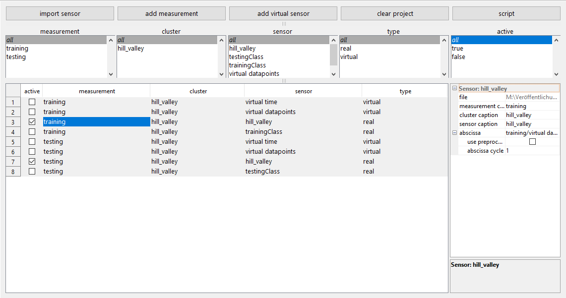
Figure 4Data import module with two measurements. All available sensors are listed in the table which can be filtered with the list boxes above. Properties of the currently selected measurement, cluster, and sensor can be edited in the PropertyTable on the right.
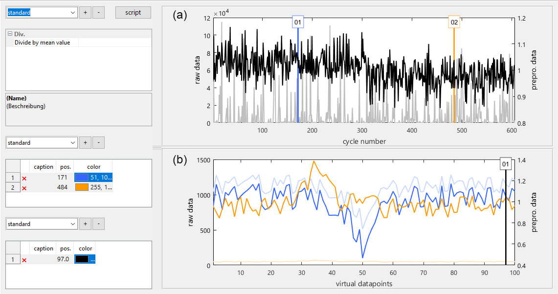
Figure 5Preprocessing module showing the quasistatic (a) and cyclic (b) view of the preprocessed data, with pale raw data in the background for comparison.
For the Hill-Valley dataset (Fig. 4), the most sensible abscissa is the sensor “virtual datapoints”. This information is only implicitly provided in the raw dataset by its matrix structure, so it makes sense to provide it as an explicit, virtual sensor for further evaluation. Two measurements are created, “training” and “testing”, so that the number of observations in the dataset is increased. Clusters and sensors must then have identical names in both measurements because DAV3E will automatically combine data of sensors with the same name only.
4.2 Preprocessing
First and foremost, the preprocessing module provides a first look on the data from two different perspectives. The upper plot shows “quasistatic” signals generated from points selected in the bottom plot. Quasistatic refers here to the fact that by always taking the sensor signal from the same point in the cycle, the resulting signal behaves like a statically operated sensor with a sampling period of one cycle length. The bottom plot, in turn, shows distinct cycles (observations) which are selected in the upper plot. Selectors in both plots can be added or deleted and moved either with the mouse or the keyboard, or by typing the desired position. They are color-coded so that a clear, visual link between the selector and the graph is established. An arbitrary number of sets can be created for the selectors in the cycle plot which generate the quasistatic signal. These sets can later be chosen for each sensor separately, which is very useful if sensors with different cycle shapes are evaluated in one dataset.
Additionally, an arbitrary number of preprocessing functions can be applied to the raw data in this module. A preprocessing function is always applied to the output data of the previous preprocessing function, which can be useful in many cases, e.g., adding an offset to data to make it nonnegative before applying the logarithm. In the example in Fig. 5, only one preprocessing function is applied. It divides each cycle by its mean value. The original data are always shown pale in the background for the user to see the impact of the current preprocessing chain. As before, several preprocessing sets can be created and assigned to sensors separately. This feature not only allows an optimal treatment of many different sensors, but also enables the user to quickly change between preprocessing methods to assess their impact on the final result.
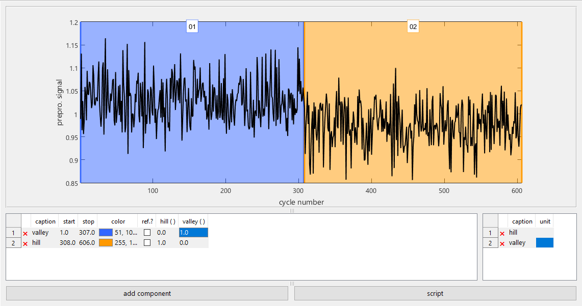
Figure 6Module to select cycle ranges which pool cycles with the same underlying conditions.
For the Hill-Valley dataset, it is obvious that the chosen preprocessing highlights differences between the classes. Valley data (from 1 to 307 in the upper plot, blue in the lower plot) tend to higher values at the end of the cycle (selected in the lower plot) than hill data (from 308 to 606 in the upper plot, orange in the lower plot). Similar differences can be seen for the beginning of the cycles, but not for the middle (not shown). In comparison to the raw data (pale in the background), this preprocessing step already provides clear differences between both classes.
4.3 Time correction
Depending on data source and hardware, a sensor signal can have a wrong offset compared to the start of the measurement, or an incorrect sampling rate. A simple example is data loaded from a CSV file with nothing but sensor data: in this case neither offset nor sample rate can be automatically determined and both are set to their defaults (0 s and 1 Hz). Failing to adjust these values can lead to erroneous results especially in combination with other sensors. The time correction module plots the quasistatic representation of one sensor of each cluster in a common graph, so that the user can immediately check whether the adjusted offset and sampling rate are correct.
4.4 Select relevant cycles
Especially in characterization measurements, often only few cycles are of interest, e.g., the cycles during which the sensor was exposed to gas or during which a certain fault was observed in a machine. While it would of course be possible to record data only during these times, it is often more convenient from an automation point of view to acquire data during the whole period of measurement. This can also be helpful to identify unexpected events in the data or drift over time, for instance. Nevertheless, usually only parts of the data are interesting for the evaluation.
This module enables easy and efficient selection and annotation of cycles of interest. The graph shows the previously determined quasistatic view for the chosen sensor. Ranges can be created, deleted, and moved by mouse or keyboard directly in the plot. Annotation means that independent states can be assigned to each range, e.g., the concentration of all test gases during each range, or, for the Hill-Valley data, whether hills or valleys are represented in this range. These annotations can later be used to create various target vectors for the model training.
The position of the ranges is internally stored as a timestamp. This allows for the correct cycle numbers to be dynamically determined for each sensor independent of its offset, sample rate, and cycle length. Thus, no resampling is necessary, which can be very resource-intensive, especially for large datasets. If two sensors with different cycle lengths are combined, resampling on a feature basis is necessary to equalize the number of observations gained from each sensor. Preliminary work to find the best resampling approach for this case has been described in Bastuck et al. (2016b).
The selection is very easy for the Hill-Valley data (Fig. 6) because the data were sorted before the import and there are no faulty or irrelevant cycles in this dataset.
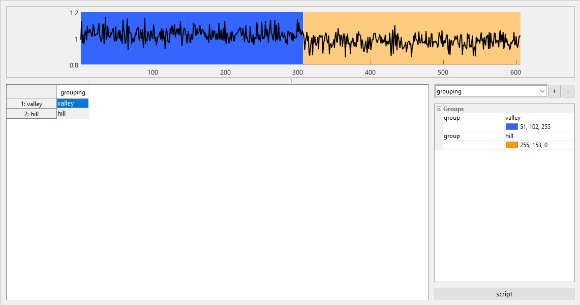
Figure 7Grouping module which is used to assign classes to the previously selected ranges. An arbitrary number of grouping vectors can be created which can later be selected as target vectors during model training. The plot shows a graphical representation of the currently selected grouping to highlight errors and to show the structure of the data at one glance.
4.5 Groupings
The grouping module is closely related to the select relevant cycles module as it uses the previously determined cycle ranges. A grouping is a vector which assigns one and only one class to each cycle range. This vector can then be expanded to a target vector that assigns a class to each cycle. The elements of the vector must be numeric if regression analysis is to be performed, but can be arbitrary strings or numbers for classification problems. Colors can be assigned to each group which are displayed in the quasistatic plot at the top, which can be helpful to discover errors in the grouping vector.
Like the range selection before, the grouping vector is trivial for the Hill-Valley dataset (Fig. 7) as for most binary classification tasks. There are usually many more options for multi-class problems, e.g., different gases with different concentrations, so that one grouping could discriminate between gases independent of concentration, while another could quantify the concentration of one gas independent of all other gases. This is discussed in detail in Sect. 5.
4.6 Feature extraction
The last step before model training is feature extraction from the cyclic data. This is a type of dimensionality reduction, considering that the number of features is reduced from, potentially, several thousand data points per cycle (depending on the sample rate) to a few features, e.g., describing the general shape. Adjacent points in a cycle are typically highly correlated, which can be problematic for many methods employed in machine learning (Næs and Mevik, 2001).
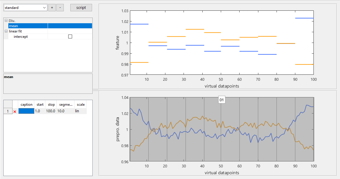
Figure 8The feature extraction module displays a representation of the average cycle shape for each group in the grouping vector. Different mathematical functions are available to summarize the points in a selected range in the cycle as one or a few values. A feature preview, here for the mean in 10 parts of the cycle, computed from the averaged cycles for speed, is shown in the top plot.
A feature is computed from the cycle with a mathematical function; features that are implemented are, for example, mean, slope, minimum and maximum values, and standard deviation. For every function, an individual set of ranges can be defined directly in the cyclic sensor signal. Thus, meaningful ranges can be selected for the respective function, e.g., long plateaus for the mean and slopes for the slope function. The ranges are defined in the bottom plot, which shows a representation of several cycles computed as the mean value of all cycles in a group of the current grouping vector. The top plot shows a preview of the current feature function applied to these mean cycles with the same colors as the examples shown in the lower plot. This kind of plot gives a first impression of the discriminating power of the selected features by visually comparing the spread between ranges, i.e., colors, that should be similar or dissimilar, respectively.
For the Hill-Valley dataset (Fig. 8), the cycle is divided into 10 equal parts for which both the mean and slope are computed; i.e., the number of features is reduced from 100 to 20. The cyclic plot (bottom) shows a significant difference between the average cycles for both classes, and the feature preview (top) confirms that the shape differences are captured by the mean feature, especially in the outermost parts as already indicated from the preprocessing; cf. Fig. 6. Distinct differences between both classes are also observed for the slope feature (not shown).
4.7 Model
The model module brings all previously defined parts of the evaluation together. Features can be selected or deselected from a list of all computed features, e.g., to observe the influence of one specific feature or feature group on the final result. The target vector for the training is defined by choosing one of the previously defined groupings. Each group's role can be determined separately, so it is possible to use a few groups for training and predict the others for model validation, or ignore groups entirely. Alternatively or additionally, a certain percentage of randomly chosen observations out of each group can be held back for testing the validated model. The model can also equalize the number of observations in each group by randomly deleting observations from larger groups. This step can significantly increase the model performance especially for small groups which would otherwise have only a small or even negligible weight in the optimization compared to large groups.
After the training data have been defined, the model-building process follows a “chain” approach very similar to the preprocessing sequence described before. One or several preprocessing steps for both features and target vectors can be applied. Note that these preprocessing functions act on the individual features and are to be distinguished from the raw data preprocessing. A typical example of feature preprocessing is rescaling the data for variance-based algorithms like PCA (van den Berg et al., 2006; Risvik, 2007), or taking the logarithm of both features and target values to model a power law, e.g., between gas sensor response and concentration (Yamazoe and Shimanoe, 2008), with the linear PLSR. Afterwards, dimensionality reduction algorithms like LDA or PCA can be applied, followed by a classifier like kNN, DA, or LR. The whole model can be validated using k-fold cross-validation or leave-one-out cross-validation. All parameters of these algorithms can be adjusted directly in the GUI, and a click on “train” performs the training and validation as defined.
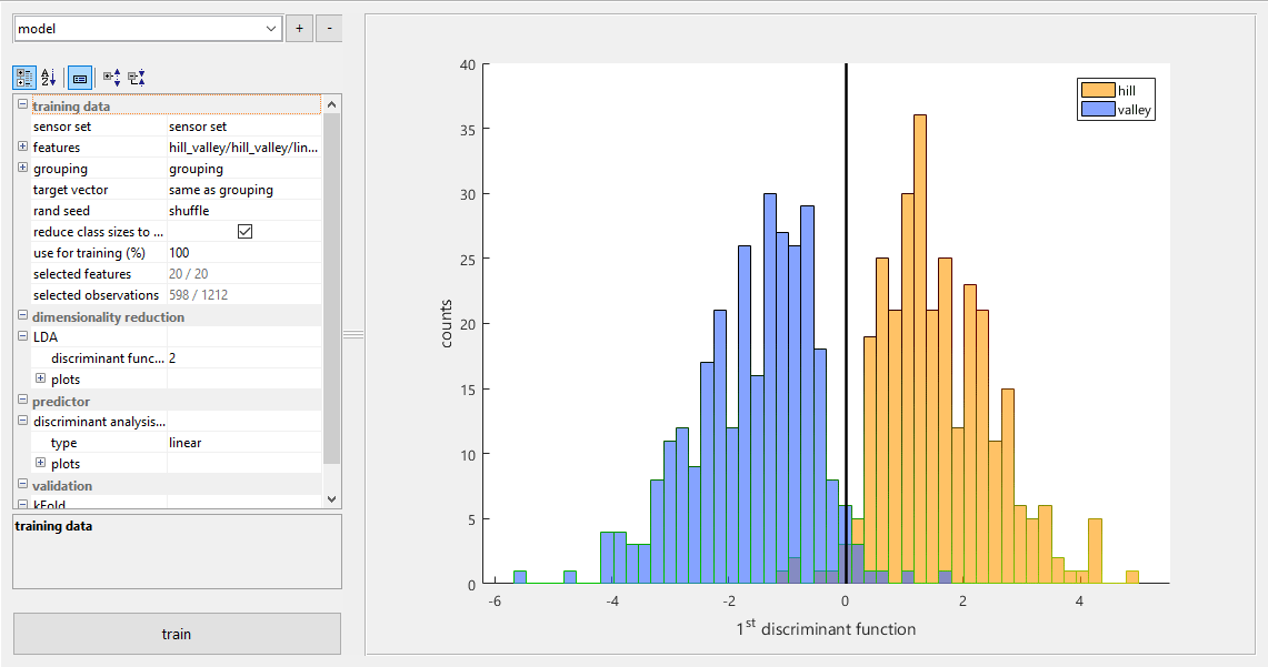
Figure 9The model module provides the possibility to exclude features or observations from the training data to see their influence on the model. In this image, the model consists of a 2-D LDA with a linear DA classifier which is validated with 10-fold cross-validation. The data distribution resulting from the dimensionality reduction is shown, with class information, as a histogram.
The results of the validation are given as classification error in percent or, for regression analysis, RMSE (root mean squared error). Additionally, many algorithms provide plots like histograms, scatter plots, or territorial plots to visualize the classification performance or areas, respectively, of the classifier in a 2-D plane. An arbitrary number of independent models can be created.
For the demonstration with the Hill-Valley dataset, a 1-D LDA is used as model (Fig. 9). The training data and classification threshold is shown in Fig. 9. Validation is done using 10-fold cross-validation (CV) and achieves a classification error of 2.5 % with all 20 features. The error increases to 5.4 % when only the 10 mean value features are used. Further inspection shows that features at the beginning and end of the cycle are the most important, so an error of 2.7 % is achieved with only eight features, i.e., means and slopes from the two outermost parts.
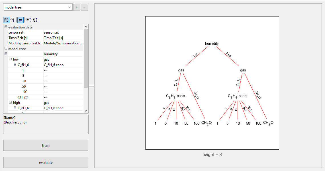
Figure 10The hierarchical model module allows for the combination of previously defined models. They can be trained with the whole dataset or only with data relevant to the model, which can lead to specialization and better results. The hierarchy is shown as a directed graph with data flow along the edges and models as nodes.
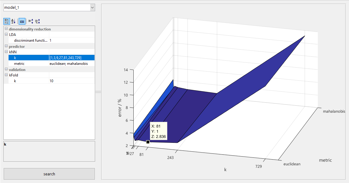
Figure 11The grid search module lists all parameters of a particular model and accepts valid MATLAB expressions as their values, so lists of values can be given for each parameter. The automated grid search evaluates the model for all permutations of parameter values and plots the model error dependent on parameter values, highlighting the optimum solution.
4.8 Model hierarchies
Classification results can often be improved with more than one model for a certain classification or quantification task (Darmastuti et al., 2015; Schütze et al., 2004). Each model can specialize or focus on a certain aspect of the task, e.g., classifying the prevalent gas with a first model and then selecting a second, specialized quantification model for this gas.
This module provides an easy interface to build such hierarchies from the previously defined models. The sensor set from which input data are taken can be defined; the data is subsequently treated according to the options for the training data given in each model separately. The previous training of the models can be used directly to predict the new data. Alternatively, the models can first be trained within the hierarchical context, in which every model splits the data according to the known classes and forwards the respective parts to the next model.
The hierarchy in Fig. 10 is an example of a gas classification and quantification task as hierarchical classification is not applicable to the Hill-Valley dataset. The behavior is often influenced by humidity, which is why the first model tries to estimate the level of humidity from the sensor data. It then forwards the data to a model specialized in gas classification in either low humidity or high humidity conditions. If benzene (C6H6) is detected, a third model is invoked, specialized in benzene quantification under either low or high humidity conditions.
4.9 Hyperparameter optimization
Finding optimal parameters for the selected model algorithms can be a complex and time-consuming task. These parameters are also called “hyperparameters” to distinguish them from the parameters that are computed by, e.g., LDA for the dimensionality reduction.
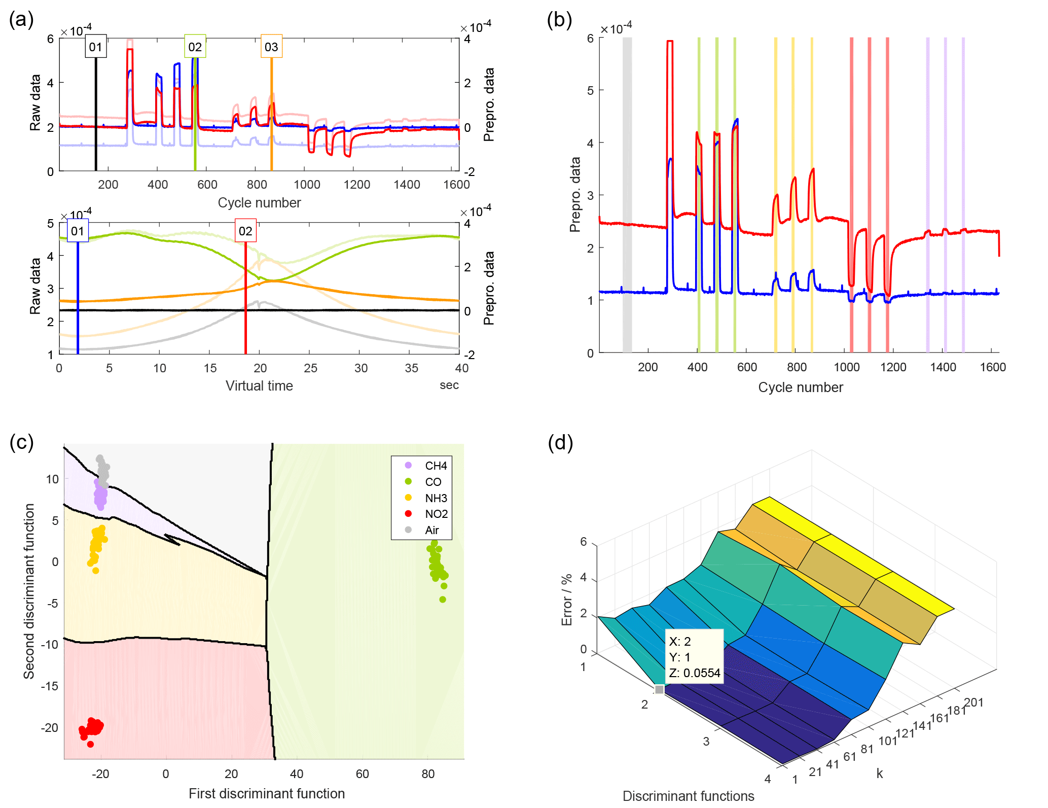
Figure 12(a) Quasistatic and cyclic signal from the UST GGS1330 gas sensor. The cycles shown are in pure air (black), CO (green), and NH3 (orange), while the quasistatic signals show the sensor reaction at low (blue) and high (red) temperature. (b) Graphical representation of a grouping for the discrimination of five classes, i.e., four gases and air. (c) Territorial plot of the resulting discrimination with the kNN classifier. (d) A grid search evaluating the model for different numbers of discriminant functions and k values of the kNN classifier.
The grid search module (Fig. 11) provides an interface in which a list of values can be given as valid MATLAB expressions for all available parameters in a model. DAV3E will then automatically perform an exhaustive search with all possible combinations of all parameter values, recording the validated model error for all combinations. After the search, the best parameter value combination is determined, and the influence of each parameter visualized.
For the Hill-Valley dataset, an exhaustive search has been performed for the parameters of a kNN classifier, i.e., the number of neighbors k (tested values: 1, 3, 9, 27, 81, 243, 729) and the metric (Euclidean or Mahalanobis distance). The search shows that k=1 and k=729 (which is actually reduced to 605, the maximum possible number of neighbors in this dataset) lead to increased error rates. This is understandable, as the result is easily negatively influenced by outliers for k=1, and each class has approximately 300 points; therefore, for k=605 the larger class will always win, which leads to many misclassifications. The distance metric's influence is almost negligible, with the Euclidean giving the optimal result of 2.8 % at k=81 for all tested parameter combinations.
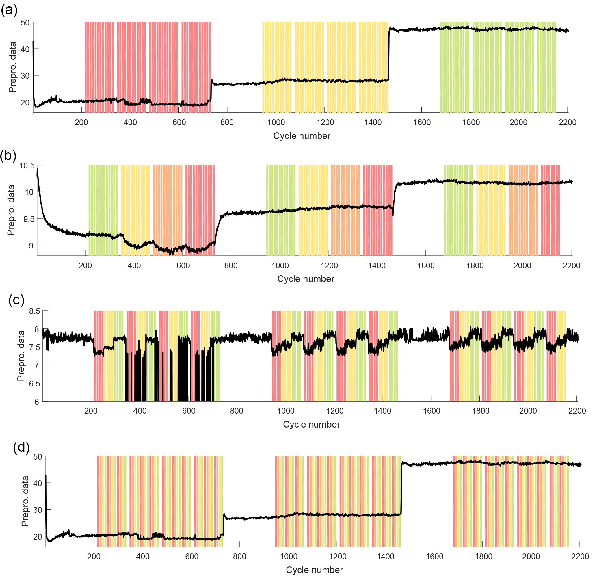
Figure 13Graphical representation of four different grouping vectors to discriminate between the severity of four different faults. Panel (a) shows three different cooler faults and the resulting cooling efficiency as a signal, and in panel (b), the pressure of the hydraulic accumulator is changed, which can be observed, e.g., in a flow sensor signal. Panel (c) shows several grades of pump leakage, evident in a different flow sensor. In (d), different grades of valve faults were experimentally simulated, which cannot be observed directly in any one individual sensor signal.
In this section, different features and aspects of DAV3E are presented for two real datasets from our research activities. All graphs shown are exported, without post-processing, directly from DAV3E. The same graphs, with all parameters, can also be automatically exported to a report document in Microsoft Word or PDF format.
5.1 Gas sensor dataset
The project described in this section is based on the dataset from Sect. 3.2. A cyclically driven gas sensor was exposed to four different gases in each of three different concentrations. Figure 12a shows the plots from the preprocessing module, i.e., quasistatic and cyclic plot. The black cycle was subtracted from all cycles, which highlights the differences in the signal shape arising from exposure to different gases. Figure 12b is a graphical representation of a grouping that discriminates between gas types, including air selected at the beginning, independent of their concentration. Other possible groupings are concentrations of one of the gases for a quantification task. These groupings can either ignore other gases, or include them explicitly as zero concentration to achieve selective quantification of a certain gas. In this dataset, the ranges can be loaded directly from the configuration file for the measurement. However, they were then shortened (using a batch script for range manipulation implemented in DAV3E) to account for fluidic time constants in the gas mixing system, resulting in approximately 10 cycles per gas exposure.
A total of 11 features are defined: the mean value of the whole cycle, and the slopes of 10 sections of equal length in the cycle.
Figure 12c is the territorial plot resulting from a 2-D LDA and a kNN classifier with Euclidean distance and k=5. Using 10-fold CV reveals a classification error of about 2.0 %, and the resulting confusion matrix identifies three points that are confused between air (gray) and methane (violet), which can already be anticipated from the plot. All other gases are identified perfectly, with distances from the air group that roughly correlate with the sensor response observed for the gas in the quasistatic plot. In contrast to all other gases, CO is a strong reduction agent and exerts more influence on the surface oxygen coverage during the cycle (Baur et al., 2015; Schultealbert et al., 2017), which leads to significant changes in the cycle shape and, thus, a shift in two dimensions instead of only one. Note that this effect is actually dominant as the CO shift is along the first discriminant axis.
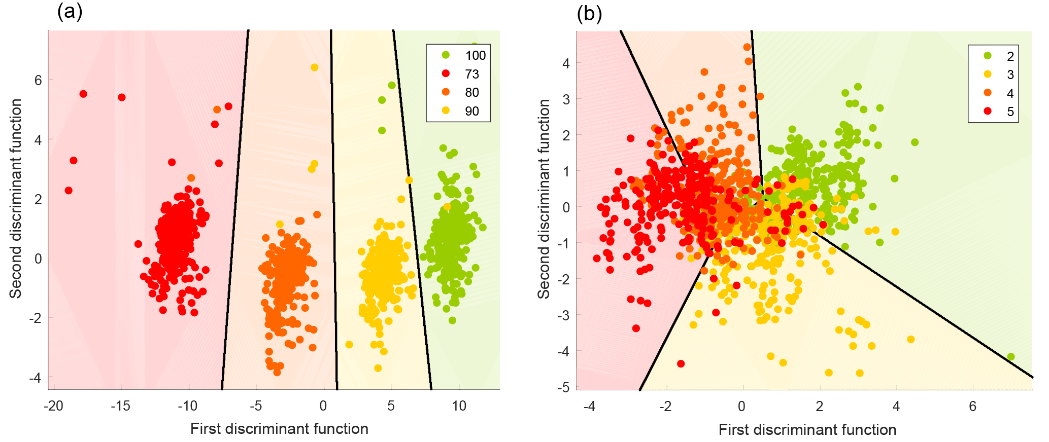
Figure 14Territorial plots of the discrimination of fault severity for (a) a valve and (b) a hydraulic accumulator.
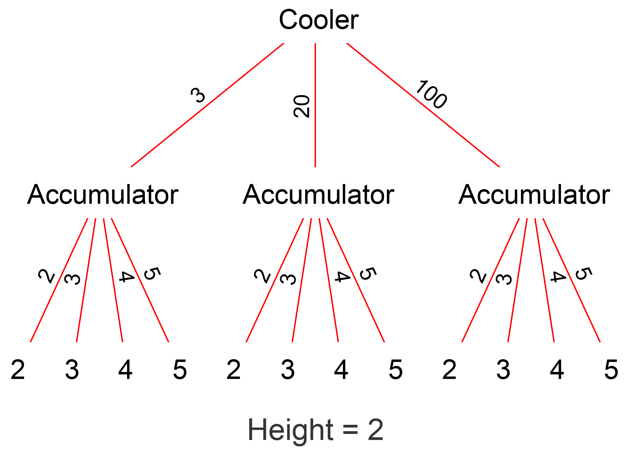
Figure 15Graph of a hierarchical model which achieves better accuracy when predicting the hydraulic accumulator fault by training specialized models for different cooling efficiencies.
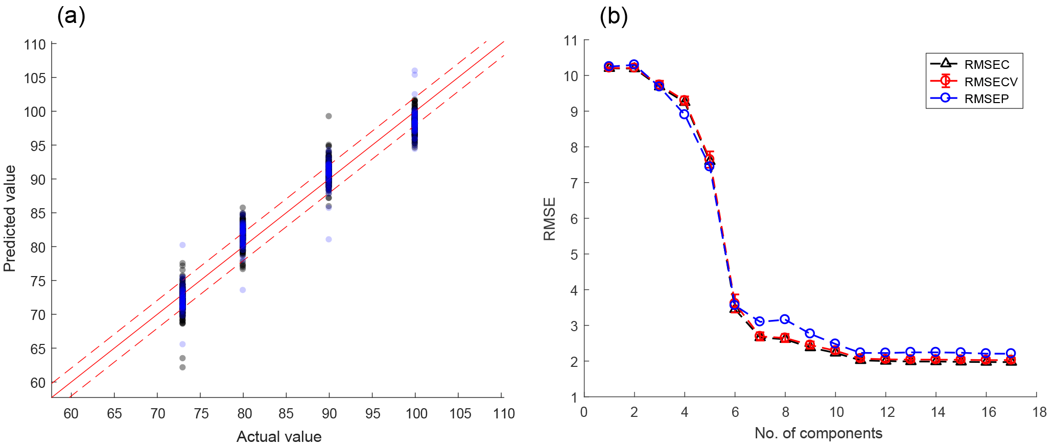
Figure 16(a) PLSR model of the valve fault with an RMSE of 2 (dashed lines), where the optimal number of components was determined with the error/component graph in (b).
In Fig. 12d, the model was evaluated for different numbers of discriminant functions and different k's for the kNN classifier. It shows that a model with only one discriminant function (DF) has a large error, which can also be understood from the territorial plot due to the significantly different effect of CO. The optimum is at two DFs and k=1. For increasing k, the error increases only slightly up to 81, which is the first time that k is greater than the sum of points in two groups. For higher k, the error increases rapidly. This is because, for equally sized classes, the correct class cannot win the decision since it is missing one point (the one under consideration) and, thus, the nearest wrong class will win.
5.2 Condition monitoring dataset
The project described in this section is based on the dataset from Sect. 3.3. A hydraulic system with a constant working cycle is monitored by 17 sensors with different sampling rates. Simulated faults and their severity are to be classified and quantified.
Figure 13 is a graphical representation of four different groupings, which are the grades of severity of four different faults, where red denotes severe, and green denotes a good condition. Panel (a) shows three grades of a cooler fault with the cooling efficiency signal which is obviously strongly influenced. As a matter of fact, the cooler efficiency has a strong influence on all 17 sensor signals and is thus a strong interfering signal that the model must ignore when other faults are to be detected. In panel (b), the pressure in the hydraulic accumulator is changed, which is observed, for example, in the signal of a flow sensor. A pump leakage is simulated in panel (c) and can be detected, amongst others, by a different flow sensor. A faulty valve is not immediately observable from any individual sensor (panel d).
For this demonstration, one feature, the mean value of the cycle, is defined per sensor, which results in a total of 17 features. The power of statistical models is shown by the fact that the valve fault, which cannot be seen in any individual sensor, can be detected almost perfectly when all features are combined (Fig. 14a; 2-D LDA, DA classifier, 0.9 % error with 10-fold CV). On the other hand, faults of the hydraulic accumulator are superimposed by cooler faults, resulting in a classification error of 35 % (Fig. 14b).
This effect can be mitigated using a hierarchical approach (Fig. 15), whereby a model first determines the severity of the cooler fault, and then forwards the data to specially trained models for detection of the accumulator fault severity at the determined cooler fault. This reduces the error from 35 % to 4 %, which improves the best result from the original paper (Helwig et al., 2015) by 6 percent points with three fewer features.
The severity of a fault and the concentration of a gas, as well as many other variables, are continuous instead of categorical. Classification methods were used here to be able to compare the results to the original paper (Helwig et al., 2015), but in general, regression methods should be used for quantification of continuous variables instead. PLSR, one of the implemented regression methods, is demonstrated in Fig. 16a for quantification of the valve fault severity. The model was built with 11 components and 80 % of the dataset. The optimal number of components can be determined with the plot in Fig. 16b, which shows the RMSEC (RMSE of calibration, black) for the training data, the RMSECV (RMSE of cross-validation, red) of a 10-fold cross-validation, and the RMSEP (RMSE of prediction, blue) for data which have not been used in training or validation. RMSEC and RMSECV are both close to 2.0 %, and the RMSEP is slightly higher with 2.2 %, which indicates that the model is able to predict previously unknown data reliably. Note that the RMSEs are given in percent because the target values are given in percent of the original valve functionality; 100 % means perfect function, whereas 73 % is close to complete failure. Hence, an RMSE of 2 % still allows an early detection of a decline of the valve's performance.
We have presented DAV3E, our MATLAB-based toolbox with GUI for building and evaluating statistical models from cyclic sensor data. Especially the feature extraction from cyclic or, more generally, time series sensor data, which can be time-consuming and hard to formalize, is lacking in current machine learning software. For a seamless workflow, DAV3E is not limited to feature extraction, but also implements many algorithms for dimensionality reduction, classification, regression, and validation, which can be extended through a simple plug-in system. Feature extraction and many other steps feature interactive plots since data visualization is becoming more and more important with the ever-increasing size of datasets. We have demonstrated several aspects of the software for three example datasets and how DAV3E was used to arrive from the raw data of many sensors to a set of statistical models for, e.g., gas classification or fault severity prediction. Many more examples can be found in our recent publications (Bastuck et al., 2016a, 2017; Leidinger et al., 2016; Sauerwald et al., 2017).
Several new functions are planned for the future, including the fusion of sensors with different cycle lengths, online prediction, and an improved grid search to test different algorithms instead of only different parameters for one algorithm.
An executable version of DAV3E can be found at http://www.lmt.uni-saarland.de/dave. The source code is available on request.
The “Hill-Valley Data Set” (Graham and Oppacher, 2008) and the dataset “Condition monitoring of hydraulic systems” (Helwig et al., 2018) are available on the UCI machine learning repository (Lichman, 2013). The dataset “Temperature-modulated gas sensor signal” is available in Bastuck and Fricke, 2018.
The supplement related to this article is available online at: https://doi.org/10.5194/jsss-7-489-2018-supplement.
MB developed and implemented the prototype DAV3E is based on. MB and TB improved upon this prototype with new ideas, concepts, and implementations. MB wrote the manuscript, and TB and AS contributed with substantial revisions.
Andreas Schütze is a member of the editorial board of the journal.
The authors would like to thank Nikolai Helwig and Thomas Fricke for kindly
providing the condition monitoring data and the gas sensor data,
respectively, Tizian Schneider for recommending the Hill-Valley dataset, and
the UCI machine learning repository for providing a platform for the
publication of machine learning datasets.
Edited by: Michele Penza
Reviewed by: two anonymous referees
Abdi, H.: Partial least squares regression and projection on latent structure regression, WIREs Comput. Stat., 2, 97–106, https://doi.org/10.1002/wics.051, 2010.
Altman, Y. M.: Undocumented Secrets of MATLAB-Java Programming, CRC Press, 2012.
Andersson, M., Pearce, R., and Spetz, A. L.: New generation SiC based field effect transistor gas sensors, Sensor. Actuat.-B Chem., 179, 95–106, https://doi.org/10.1016/j.snb.2012.12.059, 2013.
Apetrei, C., Rodríguez-Méndez, M. L., Parra, V., Gutierrez, F., and De Saja, J. A.: Array of voltammetric sensors for the discrimination of bitter solutions, Sensor. Actuat.-B Chem., 103, 145–152, https://doi.org/10.1016/j.snb.2004.04.047, 2004.
Apetrei, C., Apetrei, I. M., Nevares, I., del Alamo, M., Parra, V., Rodríguez-Méndez, M. L., and De Saja, J. A.: Using an e-tongue based on voltammetric electrodes to discriminate among red wines aged in oak barrels or aged using alternative methods. Correlation between electrochemical signals and analytical parameters, Electrochim. Acta, 52, 2588–2594, https://doi.org/10.1016/j.electacta.2006.09.014, 2007.
Bastuck, M. and Fricke, T.: Temperature-modulated gas sensor signal (Version 1.0.0), Data set, Zenodo, https://doi.org/10.5281/zenodo.1411209, 2018.
Bastuck, M., Puglisi, D., Huotari, J., Sauerwald, T., Lappalainen, J., Spetz, A. L., Andersson, M., Schütze, A., Lloyd Spetz, A., Andersson, M., and Schütze, A.: Exploring the selectivity of WO3 with iridium catalyst in an ethanol/naphthalene mixture using multivariate statistics, Thin Solid Films, 618, 263–270, https://doi.org/10.1016/j.tsf.2016.08.002, 2016a.
Bastuck, M., Baur, T., and Schütze, A.: Fusing cyclic sensor data with different cycle length, 2016 IEEE International Conference on Multisensor Fusion and Integration for Intelligent Systems (MFI), IEEE, Baden-Baden, Germany, 19–21 September 2016, 72–77, 2016b.
Bastuck, M., Daut, C., and Schütze, A.: Signalkompensation mittels Gate-Potential bei gassensitiven Feldeffekttransistoren, in 13. Dresdner Sensor-Symposium, 277–282, 2017.
Baur, T., Schütze, A., and Sauerwald, T.: Optimierung des temperaturzyklischen Betriebs von Halbleitergassensoren, tm – Tech. Mess., 82, 187–195, https://doi.org/10.1515/teme-2014-0007, 2015.
Böhm, C., Berchtold, S., and Keim, D.: Searching in high-dimensional spaces: Index structures for improving the performance of multimedia databases, ACM Comput. Surv., 33, 322–373, https://doi.org/10.1145/502807.502809, 2001.
Browne, M.: Cross-Validation Methods, J. Math. Psychol., 44, 108–132, https://doi.org/10.1006/jmps.1999.1279, 2000.
Bur, C.: Selectivity Enhancement of Gas Sensitive Field Effect Transistors by Dynamic Operation, Linköping University Electronic Press/Shaker Verlag, 2015.
Cetó, X., Apetrei, C., Del Valle, M., and Rodríguez-Méndez, M. L.: Evaluation of red wines antioxidant capacity by means of a voltammetric e-tongue with an optimized sensor array, Electrochim. Acta, 120, 180–186, https://doi.org/10.1016/j.electacta.2013.12.079, 2014.
Chang, R. M., Kauffman, R. J., and Kwon, Y.: Understanding the paradigm shift to computational social science in the presence of big data, Decis. Support Syst., 63, 67–80, https://doi.org/10.1016/j.dss.2013.08.008, 2014.
Darmastuti, Z., Bur, C., Lindqvist, N., Andersson, M., Schütze, A., and Lloyd Spetz, A.: Chemical Hierarchical methods to improve the performance of the SiC-FET as SO2 sensors in flue gas desulphurization systems, Sensor. Actuat.-B Chem., 206, 609–616, https://doi.org/10.1016/j.snb.2014.09.113, 2015.
Ding, H., Ge, H., and Liu, J.: High performance of gas identification by wavelet transform-based fast feature extraction from temperature modulated semiconductor gas sensors, Sensor. Actuat.-B Chem., 107, 749–755, https://doi.org/10.1016/j.snb.2004.12.009, 2005.
Eicker, H.: Method and apparatus for determining the concentration of one gaseous component in a mixture of gases, US Pat. 4012692, 1977.
Geladi, P. and Kowalski, B. R.: Partial least-squares regression: a tutorial, Anal. Chim. Acta, 185, 1–17, https://doi.org/10.1016/0003-2670(86)80028-9, 1986.
Graham, L. and Oppacher, F.: Hill-Valley Data Set, UCI Machine Learning Repository, 2008, available at: http://archive.ics.uci.edu/ml/datasets/hill-valley, last access: 14 September 2018.
Gramm, A. and Schütze, A.: High performance solvent vapor identification with a two sensor array using temperature cycling and pattern classification, Sensor. Actuat.-B Chem., 95, 58–65, https://doi.org/10.1016/S0925-4005(03)00404-0, 2003.
Gutierrez-Osuna, R.: Pattern analysis for machine olfaction: A review, IEEE Sens. J., 2, 189–202, https://doi.org/10.1109/JSEN.2002.800688, 2002.
Gutierrez-Osuna, R. and Nagle, H. T.: A method for evaluating data-preprocessing techniques for odor classification with an array of gas sensors, IEEE T. Syst. Man Cy. B, 29, 626–632, https://doi.org/10.1109/3477.790446, 1999.
Hastie, T., Tibshirani, R., and Friedman, J.: The Elements of Statistical Learning, Springer, 2009.
Hawkins, D. M.: The Problem of Overfitting, J. Chem. Inf. Comput. Sci., 44, 1–12, https://doi.org/10.1021/ci0342472, 2004.
HDF5 Group: HDF5, available at: https://www.hdfgroup.org/HDF5/, last access: 13 February 2016.
Heilig, A., Bârsan, N., Weimar, U., Schweizer-Berberich, M., Gardner, J. W., and Göpel, W.: Gas identification by modulating temperatures of SnO2-based thick film sensors, Sensor. Actuat.-B Chem., 43, 45–51, https://doi.org/10.1016/S0925-4005(97)00096-8, 1997.
Helwig, N., Schüler, M., Bur, C., Schütze, A., and Sauerwald, T.: Gas mixing apparatus for automated gas sensor characterization, Meas. Sci. Technol., 25, 055903, https://doi.org/10.1088/0957-0233/25/5/055903, 2014.
Helwig, N., Pignanelli, E., and Schütze, A.: Condition monitoring of a complex hydraulic system using multivariate statistics, 2015 IEEE International Instrumentation and Measurement Technology Conference (I2MTC) Proceedings, 210–215, https://doi.org/10.1109/I2MTC.2015.7151267, 2015.
Helwig, N., Pignanelli, E., and Schütze, A.: Condition monitoring of hydraulic systems Data Set, UCI Machine Learning Repository, 2018, available at: https://archive.ics.uci.edu/ml/datasets/Condition+monitoring+of+hydraulic+systems, last access: 14 September 2018.
Huang, X. J., Choi, Y. K., Yun, K. S., and Yoon, E.: Oscillating behaviour of hazardous gas on tin oxide gas sensor: Fourier and wavelet transform analysis, Sensor. Actuat.-B Chem., 115, 357–364, https://doi.org/10.1016/j.snb.2005.09.022, 2006.
James, G., Witten, D., Hastie, T., and Tibshirani, R.: An introduction to statistical learning: with applications in R, Springer, 2013.
Kitchin, R.: Big Data, new epistemologies and paradigm shifts, Big Data Soc., 1, 1–12, https://doi.org/10.1177/2053951714528481, 2014.
Kohavi, R.: A Study of Cross-Validation and Bootstrap for Accuracy Estimation and Model Selection, IJCAI'95 Proceedings of the 14th international joint conference on Artificial intelligence, 14, 1137–1143, 1995.
Lee, A. P. and Reedy, B. J.: Temperature modulation in semiconductor gas sensing, Sensor. Actuat.-B Chem., 60, 35–42, https://doi.org/10.1016/S0925-4005(99)00241-5, 1999.
Leidinger, M., Huotari, J., Sauerwald, T., Lappalainen, J., and Schütze, A.: Selective detection of naphthalene with nanostructured WO3 gas sensors prepared by pulsed laser deposition, J. Sens. Sens. Syst., 5, 147–156, https://doi.org/10.5194/jsss-5-147-2016, 2016.
Lichman, M.: UCI Machine Learning Repository, Univ. California, Irvine, Sch. Inf. Comput. Sci., available at: http://archive.ics.uci.edu/ml (last access: 14 September 2018), 2013.
Marco, S. and Gutierrez-Galvez, A.: Signal and data processing for machine olfaction and chemical sensing: A review, IEEE Sens. J., 12, 3189–3214, https://doi.org/10.1109/JSEN.2012.2192920, 2012.
Moreno-Barón, L., Cartas, R., Merkoçi, A., Alegret, S., Del Valle, M., Leija, L., Hernandez, P. R., and Muñoz, R.: Application of the wavelet transform coupled with artificial neural networks for quantification purposes in a voltammetric electronic tongue, Sensor. Actuat.-B Chem., 113, 487–499, https://doi.org/10.1016/j.snb.2005.03.063, 2006.
Næs, T. and Mevik, B. H.: Understanding the collinearity problem in regression and discriminant analysis, J. Chemom., 15, 413–426, https://doi.org/10.1002/cem.676, 2001.
Reimann, P. and Schütze, A.: Sensor Arrays, Virtual Multisensors, Data Fusion, and Gas Sensor Data Evaluation, in Gas Sensing Fundamentals, vol. 15, edited by: Kohl, C.-D. and Wagner, T., Springer Berlin Heidelberg, Berlin, Heidelberg, 67–107, 2014.
Risvik, H.: Principal component analysis (PCA) & NIPALS algorithm, 2007.
Sampson, D. and Tordoff, B.: GUI Layout Toolbox, available at: https://de.mathworks.com/matlabcentral/fileexchange/47982-gui-layout-toolbox, last access: 28 January 2017.
Sauerwald, T., Baur, T., Leidinger, M., Spinelle, L., Gerboles, M., and Schütze, A.: Laborübertragbare Kalibrierung von Sensoren für die Messung von Benzol, 13. Dresdner Sensor-Symposium, Dresden, Germany, 4–6 Dezember, 2017, 105–110, 2017.
Schultealbert, C., Baur, T., Schütze, A., Böttcher, S., and Sauerwald, T.: A novel approach towards calibrated measurement of trace gases using metal oxide semiconductor sensors, Sensor. Actuat.-B Chem., 239, 390–396, https://doi.org/10.1016/j.snb.2016.08.002, 2017.
Schütze, A., Gramm, A., and Rühl, T.: Identification of organic solvents by a virtual multisensor system with hierarchical classification, IEEE Sens. J., 4, 857–863, https://doi.org/10.1109/JSEN.2004.833514, 2004.
Smola, A. J. and Schölkopf, B.: A tutorial on support vector regression, Stat. Comput., 14, 199–222, https://doi.org/10.1023/B:STCO.0000035301.49549.88, 2004.
van den Berg, R. a, Hoefsloot, H. C. J., Westerhuis, J. a, Smilde, A. K., and van der Werf, M. J.: Centering, scaling, and transformations: improving the biological information content of metabolomics data, BMC Genomics, 7, 142, https://doi.org/10.1186/1471-2164-7-142, 2006.
Winquist, F., Wide, P., and Lundström, I.: An electronic tongue based on voltammetry, Anal. Chim. Acta, 357, 21–31, https://doi.org/10.1016/S0003-2670(97)00498-4, 1997.
Yamazoe, N. and Shimanoe, K.: Theory of power laws for semiconductor gas sensors, Sensor. Actuat.-B Chem., 128, 566–573, https://doi.org/10.1016/j.snb.2007.07.036, 2008.