3.1 General aspects on synthetic aperture imaging of heterogeneous media

Since synthetic aperture (SA) data are time- and space-dependent, the data processing can operate in the time and space domain or in the temporal and spatial frequency domain, which is obtained from a multidimensional Fourier transform of the measured data. A straightforward way to compress the SA data is by employing matched filtering in the time–space domain (Cumming and Wong, 2005). Here, for each pixel, that is, each possible target ${\mathit{r}}_{\mathrm{T},i}=$ (x_T,i, y_T,i, z_T,i)^T, a signal hypothesis is stated. This hypothesis equals the signal which the antenna at position ${\mathit{r}}_{\mathrm{A},j}=$ (x_A,j, y_A,j, z_A,j)^T would receive if there was a point scatterer located in the point r_T,i. In a next step, the hypotheses $s_{\mathrm{R}x,\mathrm{hyp},ij}\left({\mathit{r}}_{\mathrm{T},i},{\mathit{r}}_{\mathrm{A},j},f,t\right)$ are correlated with the actually measured signal $s_{\mathrm{R}x,\mathrm{meas},j}\left({\mathit{r}}_{\mathrm{A},j},f,t\right)$ at the current antenna position.

Here, η denotes the shift of the correlation integral. Those points in which a scattering truly occurs will then exhibit a high value for the correlation. All other points will exhibit a low value. Finally, in each voxel the values of the correlation function ψ_ij for all N_A antenna positions r_A,j, jϵ[1,N_A] and, in the case of a multi-frequency system, all N_f frequency steps f_m, mϵ[1,N_f], are summed up:

The resulting absolute value of the complex phasor ψ_sum,i is a measure of the probability that a point scatterer will be located in the respective point r_T,i. Converting the resulting absolute values of all N_T voxels r_T,i, iϵ[1,N_T] to brightness values returns the reconstructed image. That way, due to the pixel-wise filtering a precise compression of the targets can be obtained. However, it is obvious that this approach performs poorly in terms of computing time. This is especially true in the field of subsurface imaging: for the matched filtering, the path traversed by the wave needs to be known. In a heterogeneous surrounding, the wave will be refracted according to Eq. (6). However, the two angles α and β are not known a priori due to the unfocused antennas used for SAR. Therefore, the algorithm first has to determine the wave's path and then can proceed to the correlation procedure described above.

There is a number of reconstruction algorithms employed for SAR processing, like range-Doppler, chirp scaling or ω-k, which operate partly or entirely in the frequency domain (Cumming and Wong, 2005). In their original form they were based on the assumption of free-space propagation of the waves, but they have been adapted to inhomogeneous surroundings in past years (Albakhali and Moghaddam, 2009; Skjelvareid et al., 2011). However, in most cases the adapted algorithms can only handle planar objects. Some methods have been proposed which are also suitable for non-planar objects (Qin et al., 2014), but they require iterative processing steps, which considerably reduces their efficiency.

Therefore, matched filtering, which can be applied to any geometry, is still the most commonly used technique for subsurface imaging of irregularly shaped objects and will be used in this contribution, too.

3.2 Contour detection

If the contour of the object, which is the material boundary between the two media, is not known – or if it is known but its orientation towards the aperture plane is not – then the material boundary must be determined prior to the actual reconstruction. In the following, a way to extract the contour directly from the measurement data is shown.

Therefore, we first reconstruct the space between the aperture and the boundary. Here we can assume a free-space propagation of the EM wave, which means that no refraction has to be taken into account. The resulting image will be defocused, but the boundary will be reconstructed at its true position. Since the boundary will be the strongest reflection in most cases, one way to extract it directly is to search for the brightest pixel in each column. This approach is often used in ground-penetrating radar (Walker and Bell, 2001; Feng et al., 2010). It is convenient because it does not require additional measurements and there are effective algorithms existing for a free-space reconstruction.

Evidently however the error made in estimating the boundary will affect the quality (i.e. the signal-to-noise ratio, SNR) of the further reconstruction: due to the imaging principle of interfering single measurements it is essential that the resulting phase error caused by the estimation uncertainty is less than ±90^∘ in order to avoid destructive interference.

3.3 Refraction ray tracing

This section addresses the matched filtering for heterogeneous surroundings. A model of the scenario with the applied nomenclature is shown in Fig. 1. Here, the indices A, T, and B denote the coordinates of the respective antenna, boundary point and target. For clarity the indices i, j and m utilized in Sect. 3.1 are left out. The lateral (azimuth) direction is x; the range direction is z. For the sake of simplicity, all considerations are derived for a 2-D set-up.

We use a monostatic synthetic aperture radar, transmitting a signal s_Tx(tf). The receiver signal s_Rx(tf) is the wave backscattered from the DUT. The antenna positions spanning the synthetic aperture are equidistantly spaced and they are located at z=0. The antenna itself is modelled as an isotropic radiator. It is presumed that the volume to be reconstructed is located in the antenna's far-field. Then, the spherical wave radiated from the antenna will intersect with the object only at a small section of the sphere. This small section can be approximated as a quasi-plane phase front. Therefore, we model the incident wave to be a plane wave.

Figure 1Model and nomenclature.

Download

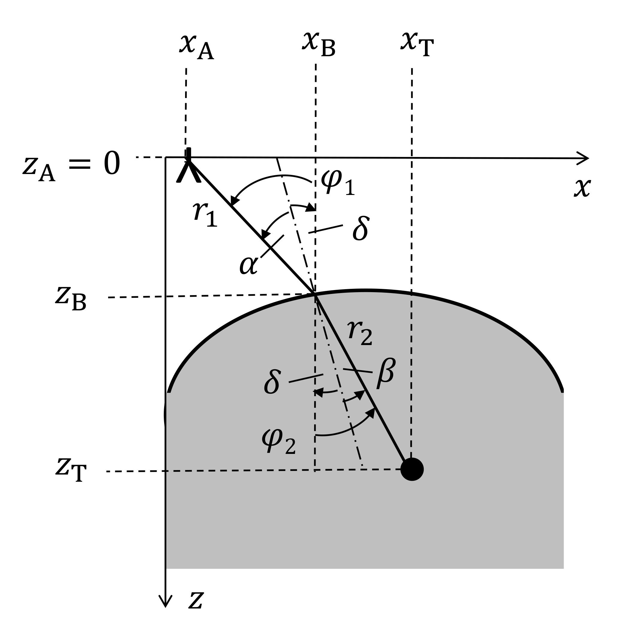
According to the antenna's isotropic directivity pattern, some part of the radiated electromagnetic field will be radiated in such a way that after traversing medium one and being refracted at the boundary it will actually meet the target (r₁ and r₂ in Fig. 1). Assuming isotropic scattering, some part of the reflected field will traverse the same way back to the antenna. Then, the received signal's phase will be

which follows from Eqs. (2) to (5).

In Eq. (11), any phase offset due to the scatterer's reflection properties will be neglected, for it is a constant and thus will not influence the reconstruction process. Furthermore, since the reconstruction method will only evaluate the phase, the signal's amplitude is not considered further. Accordingly, the signal hypothesis becomes

when setting the amplitude to a virtual value of one and inserting Eq. (11) for the phase.

Throughout this article we assume the object under test to consist of one non-magnetic, dielectric, frequency-independent and lossless material whose electric permittivity is known. For many NDT applications these are valid assumptions.

In the following, two means of finding the optical path in a two-media system are described. One is based on Snell's law, and the other one is based on Fermat's principle.

4.1 Measurement set-up

Measurements were conducted to demonstrate the algorithm's feasibility. Here, we examined a polyethylene (PE) object into which two holes were drilled. Polyethylene displays a relative permittivity of ε_r = 2.3 in the relevant frequency range (Elvers, 2016). The drill holes represent air inclusions within the material. Such imperfections can be caused in the production process of the polymer or in the operation of a component.

The object under test is depicted in Fig. 3. It was constructed to be invariant along the vertical direction, thus allowing for a 2-D reconstruction. Its surface was chosen to be non-planar and non-symmetric in order to demonstrate the algorithm's capacity to reconstruct rather complex objects.

Figure 2Flowchart of the image reconstruction process.

Download

Figure 3Sketch of the object under test and its cross section with all relevant measures.

Download

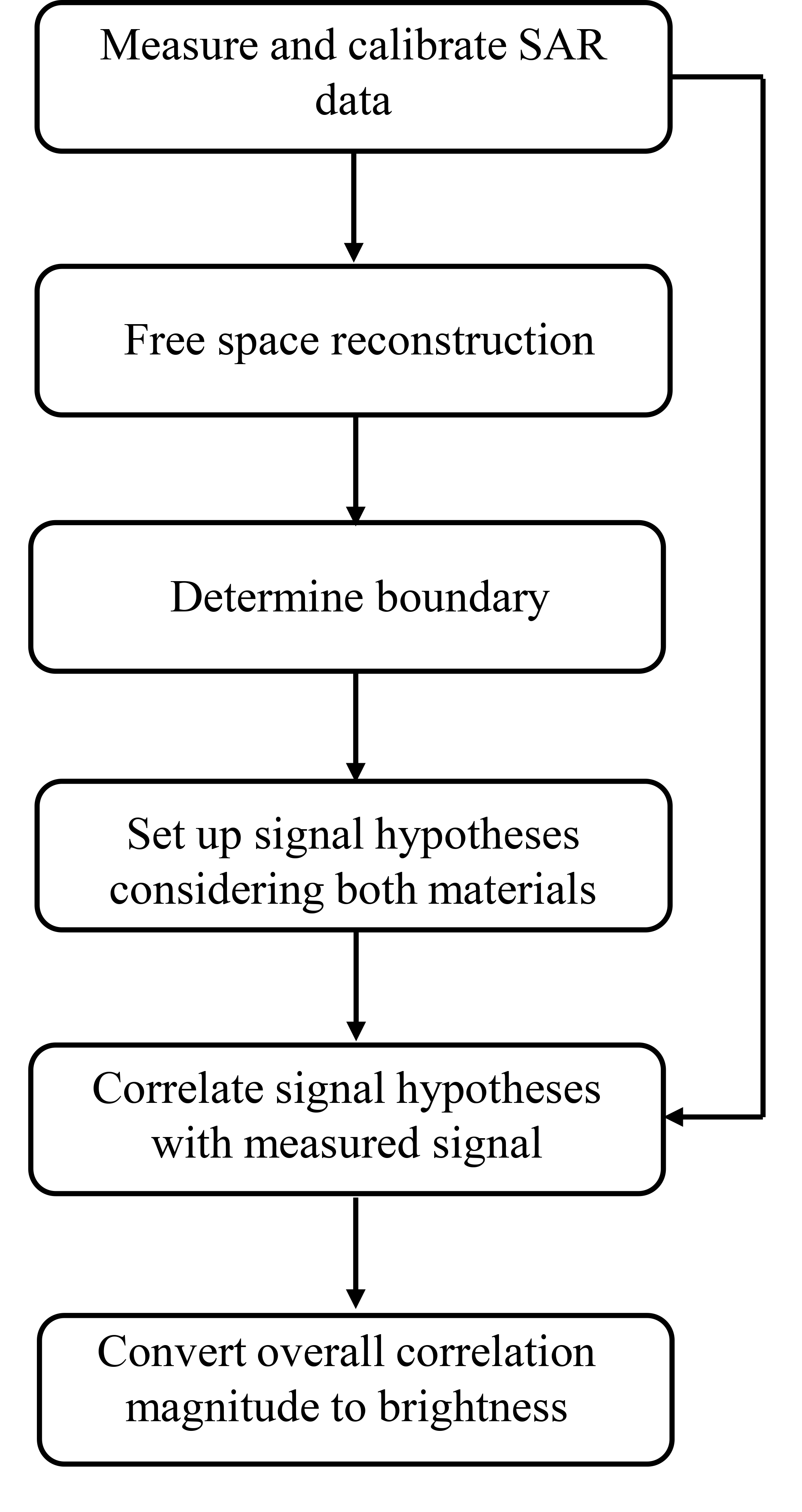
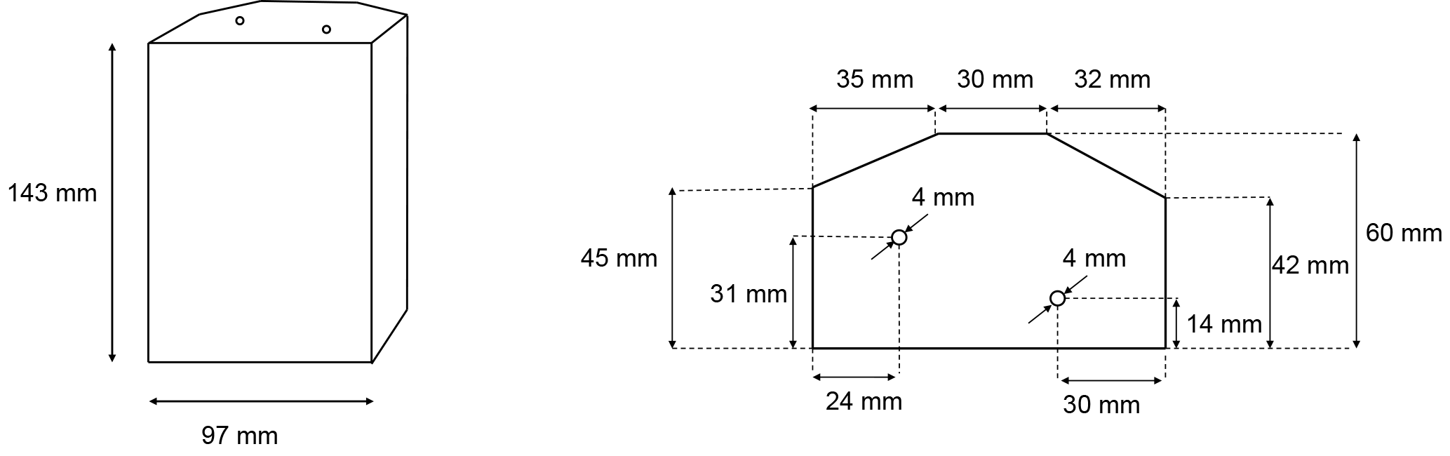
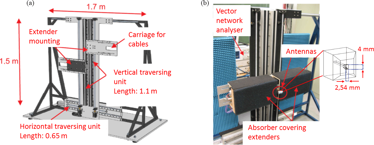
Figure 4Employed measurement set-up. (a) Set-up sketch; (b) photograph of the measuring unit with an enlarged sketch of one of the antennas (Gumbmann, 2011).

Download

Table 1Measurement parameters.

Download Print Version | Download XLSX

The employed measurement set-up is shown in Fig. 4. It consists of one horizontal and two vertical traversing units, on which a pair of antennas is mounted. The traversing units allow for a movement along a distance of approximately 1.1 m in the vertical direction and 0.65 m in the horizontal direction. It is therefore possible to span a synthetic aperture of those dimensions. The two vertical units can be moved separately, which also makes multistatic measurements possible. For the measurements presented in this paper we employed a quasi-monostatic set-up, i.e. transmitter and receiver antenna were in close proximity; they were mounted with a spacing of 2 mm between them. The antennas were two H-polarized horn antennas with a physical aperture of 2.45 mm × 4 mm (see Fig. 4). The transmitted signal was generated by a vector network analyser (Agilent PNA E8363B) with frequency extenders (Oleson Microwave Labs V10VNA2-T/R). A 201-point SFCW signal covering the complete W-band (frequency range: $f_{min}=\mathrm{75}$ GHz to $f_{max}=\mathrm{110}$ GHz) was employed. Accordingly, the corresponding free-space wavelengths cover a range from λ_min = 2.7 mm to λ_max = 4 mm and a bandwidth of B = 35 GHz can be used. This bandwidth and wavelengths allow for a resolution in the range of a few millimetres, as will be discussed in Sect. 4.2. The radiated power was P_Tx = −17 dBm (20 µW).

In order to generate a 2-D image, a line aperture is sufficient. From the spatial sampling theorem the spacing between the antenna array positions must not exceed

(Benetsy et al., 2008), which is 1.35 mm for the W-band. Here, a spacing of 1 mm was chosen. The total length of the line aperture was L_Ap = 400 mm. The PE test object was positioned in such a way that its front plateau (see Fig. 3) was orientated parallel to the line aperture at a distance of $z_{min}=\mathrm{25.8}$ cm. Thus, the field of view of the reconstructed image needs to reach up to $z_{max}=\mathrm{31.8}$ cm in the range direction (see Fig. 3). Table 1 sums up the parameters of the measurements.

The system is calibrated by two calibration measurements (Gumbmann, 2011):

• Load standard: an empty space measurement with no reflecting object to eliminate crosstalk between the antennas;

• short standard: a measurement with a metal plate placed in front of the aperture at a defined reference distance d_ref to eliminate the frequency response of the components (network analyser, extenders, antennas and cables).

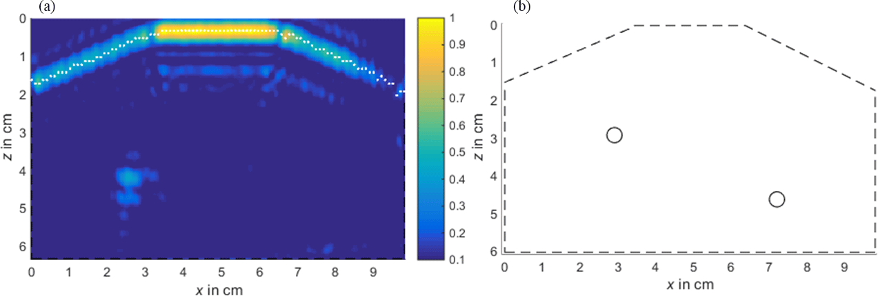
Figure 5(a) Free-space reconstruction and detected object contour (white); (b) ideal geometry sketch of the object under test.

Download

The raw data s_Rx,raw were then calibrated by

Here, s_Rx,load and s_Rx,short are the data obtained from the two calibration measurements named above. The notation 〈⋅〉 symbolizes the mean value over a number of measurements (10 in the presented experiments). The factor −1 is the reflection coefficient of the short. The reference phase φ_ref is the phase calculated from the short measurement. It is

4.2 Results

As a first step, a free-space reconstruction of the calibrated data was performed. Figure 5 shows the reconstruction of the object assuming free-space propagation throughout the whole domain. As a reference for the reconstructed image, a sketch of the DUT's geometry is depicted also. For the sake of simplicity, the object is depicted in a local coordinate system, starting from z=0 at the DUT's front boundary. In the global coordinate system, the object was located at a range of 25.8 cm from the aperture line, as mentioned above. It can be seen that the target at z ≈ 4.5 cm is not depicted within the object. The lower boundary is not visible either. The image is rather defocused, too.

The reconstruction image is normalized to its maximum intensity value. For clutter reduction, all pixels exhibiting a value below 10 % of the maximum value are set to zero. The object's contour is illustrated by dashed lines.

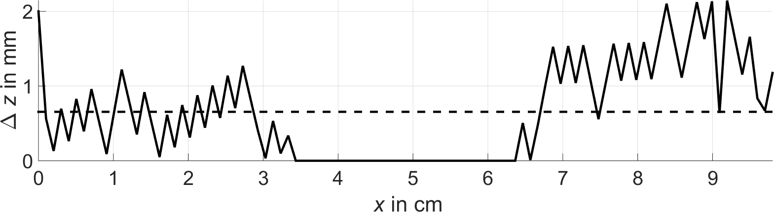
The boundary contour was estimated by a column-wise maximum search as described in Sect. 3.2. The respective points are depicted in white in Fig. 5. For a comparison the estimated boundary is shown in Fig. 6 together with the true contour. It can be seen that the estimation is a good approximation to the real contour: on the upper plateau the estimated values and the analytical ones match perfectly. The error made by the estimation is depicted in Fig. 7. Its mean value is 0.655 mm; the maximum error is 2.14 mm. The estimation displays an uncertainty that is determined by the system's range resolution. For the W-band, whose bandwidth B is 35 GHz, it is

in free space.

Figure 8 shows the image obtained with the described material-sensitive reconstruction algorithm based on the estimated material boundary. Here, Fermat's principle was used for the ray tracing. The concept based on Snell's law was evaluated in the conference paper (Ullmann et al., 2017). Again, the image is normalized to the maximum intensity and all values below 0.1 are neglected. As before, the reference sketch can be seen on the right side of the figure.

Figure 6Comparison of the detected material boundary (solid line) and its analytical contour (dashed line).

Download

Figure 7Estimation error Δz for the material boundary. Dashed line: mean error.

Download

Figure 8(a) Reconstructed image with estimated boundary (white); (b) ideal geometry sketch.

Download

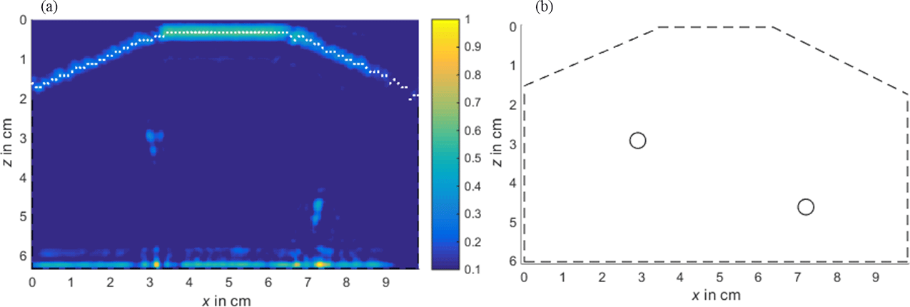
Note that in the reconstructed images only the targets' upper and lower boundaries are visible. They correspond to the material discontinuities at which reflections occur. From Fig. 8 it can be seen that in contrast to the free-space reconstruction, both targets are reconstructed at their true positions. The improvement in the localization is because in the free-space case the propagation velocity is assumed too high. Consequently, since the velocity is proportional to the traversed way, an overly long distance along the range direction is reconstructed. With the adapted algorithm this error is not made. Furthermore, with the developed method the targets and the material boundary are focused more precisely. Since the lateral resolution depends on the wavelength λ, the aperture length L_Ap and the distance z between the aperture plane and the depicted position

and the range resolution depends on bandwidth and phase velocity (see Eq. 24), a better resolution can be obtained when taking the material characteristics, which affect the phase velocity and the wavelength, into account. From Eqs. (24) and (25) and Table 1 it can be seen that a resolution with theoretical limits of δ_r=2.84 mm in the range direction and δ_lat= 1.04 mm in the lateral direction can be obtained with the described set-up.

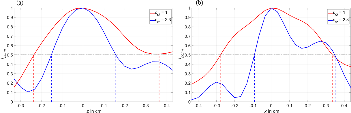
Figure 9Comparing the resolution of free-space reconstruction (ε_r2 = 1) and material-sensitive reconstruction (ε_r2 = 2.3) on the upper target. (a) Range resolution; (b) lateral resolution.

Download

The actual resolution in the reconstructed images can be estimated from Fig. 9. Here, the point that displayed the maximum intensity at the upper left air inclusion (x ≈ 2.5) was picked out from the datasets depicted in Figs. 5 and 8. The range and lateral resolution can then be estimated by finding the distance Δz or Δx, respectively, between the two points of half the maximum intensity. They are depicted by dashed lines in Fig. 9. For the sake of simplicity and because their z-values do not match, as described previously, the curves are normalized to a dimensionless maximum intensity of 1 and the x-/z-coordinate of the maximum point was set to 0. It can be seen from Fig. 9 that the material-sensitive reconstruction (blue curve) displays a smaller (i.e. higher) resolution in both the range and lateral directions compared to the free-space reconstruction (red curve). Note however that in the material-sensitive reconstruction the upper target is reconstructed by two rather than one point of high intensity (see Fig. 8). This is because the hole with a diameter of 4 mm does not represent a point target for the employed system. Consequently, in Fig. 9 there are two peaks rather than one, and they are overlapping, so that a proper determination of the resolution is difficult.

From Fig. 9 the respective resolutions can be estimated to

• δ_r= 5.99 mm in the free-space reconstruction versus δ_r= 3.08 mm in the material-sensitive reconstruction;

• δ_lat= 6.13 mm in the free-space reconstruction versus δ_lat= 4.26 mm in the material-sensitive reconstruction.

Note that, when instead examining the lower right target (x ≈ 7.5), a lateral resolution of approximately 2.2 mm can be estimated for the material-sensitive reconstruction in the same way as before. Noise as well as the error caused by the boundary estimation are possible reasons for the deviation between the theoretically achievable and practically achieved resolutions.