the Creative Commons Attribution 4.0 License.
the Creative Commons Attribution 4.0 License.
 | 16 Apr 2018
Temperature estimation of induction machines based on wireless sensor networks
Yi Huang
Clemens Gühmann
In this paper, a fourth-order Kalman filter (KF) algorithm is implemented in the wireless sensor node to estimate the temperatures of the stator winding, the rotor cage and the stator core in the induction machine. Three separate wireless sensor nodes are used as the data acquisition systems for different input signals. Six Hall sensors are used to acquire the three-phase stator currents and voltages of the induction machine. All of them are processed to root mean square (rms) in ampere and volt. A rotary encoder is mounted for the rotor speed and Pt-1000 is used for the temperature of the coolant air. The processed signals in the physical unit are transmitted wirelessly to the host wireless sensor node, where the KF is implemented with fixed-point arithmetic in Contiki OS. Time-division multiple access (TDMA) is used to make the wireless transmission more stable. Compared to the floating-point implementation, the fixed-point implementation has the same estimation accuracy at only about one-fifth of the computation time. The temperature estimation system can work under any work condition as long as there are currents through the machine. It can also be rebooted for estimation even when wireless transmission has collapsed or packages are missing.


Electrical machines are widely used in the industry, especially with the increasing interest in electric and hybrid electric vehicles. The thermal behavior of an induction machine largely determines the maximum lifetime, to cope with overload conditions and also the accuracy in a high-performance controller (Sonnaillon et al., 2010). Normally, three methods are used for the temperature monitoring. The most common method is the measurement by construction of a temperature measurement system using a mounted sensor. Even the rotor temperature can be measured by a wireless sensor network (WSN) (Ben Brahim et al., 2016; Brahim et al., 2016), or by some optimized optical fiber sensors (Hudon et al., 2016; Wang et al., 2009). An indirect approach is the temperature calculation based on the estimation of resistive parameters. Based on the stator windings resistance variation with temperature, a sensorless internal temperature monitoring method for an induction motor is introduced (Sabaghi et al., 2007). Thermal analysis based on a lumped-parameter thermal network (Haumer et al., 2012) is a third way which can be used for the temperature monitoring directly.
Meanwhile the WSNs have many applications, such as industry, environment monitoring, tracking of things and internet of things. A number of methods for temperature monitoring of induction machines can be found in the literature. Some of the methods do not provide satisfying results or can only estimate the temperatures of stator winding and rotor cages without a stator core (Ozsoy et al., 2010). Other methods require powerful computation capabilities which cannot be run on a resource-limited node.
In conclusion, many of the monitoring applications for the electrical machine based on a WSN can be found in the literature. However, none of them has implemented a temperature estimation algorithm on a resource-limited wireless sensor node. The temperature monitoring system of an induction machine based on a WSN is explored in this paper. We focus on the algorithmic implementation on the wireless sensor network. The input signal is the processing of the signals of a single node distributed over different nodes and transmitted to the host node, where the algorithm is implemented. Section 2 gives a description of the system. The implementation of a wireless transducer interface module (WTIM) and a network capable application processor (NCAP, IEE, 2007a) is described in Sects. 3 and 4. The communication of the WSN system is described in Sect. 5. Experimental results are discussed in Sect. 6 and the conclusions are followed in Sect. 7.
2.1 The thermal model of the asynchronous machines
The thermal network of the machine can be summarized as the following Fig. 1, which is based on the thermal model (Haumer et al., 2012).
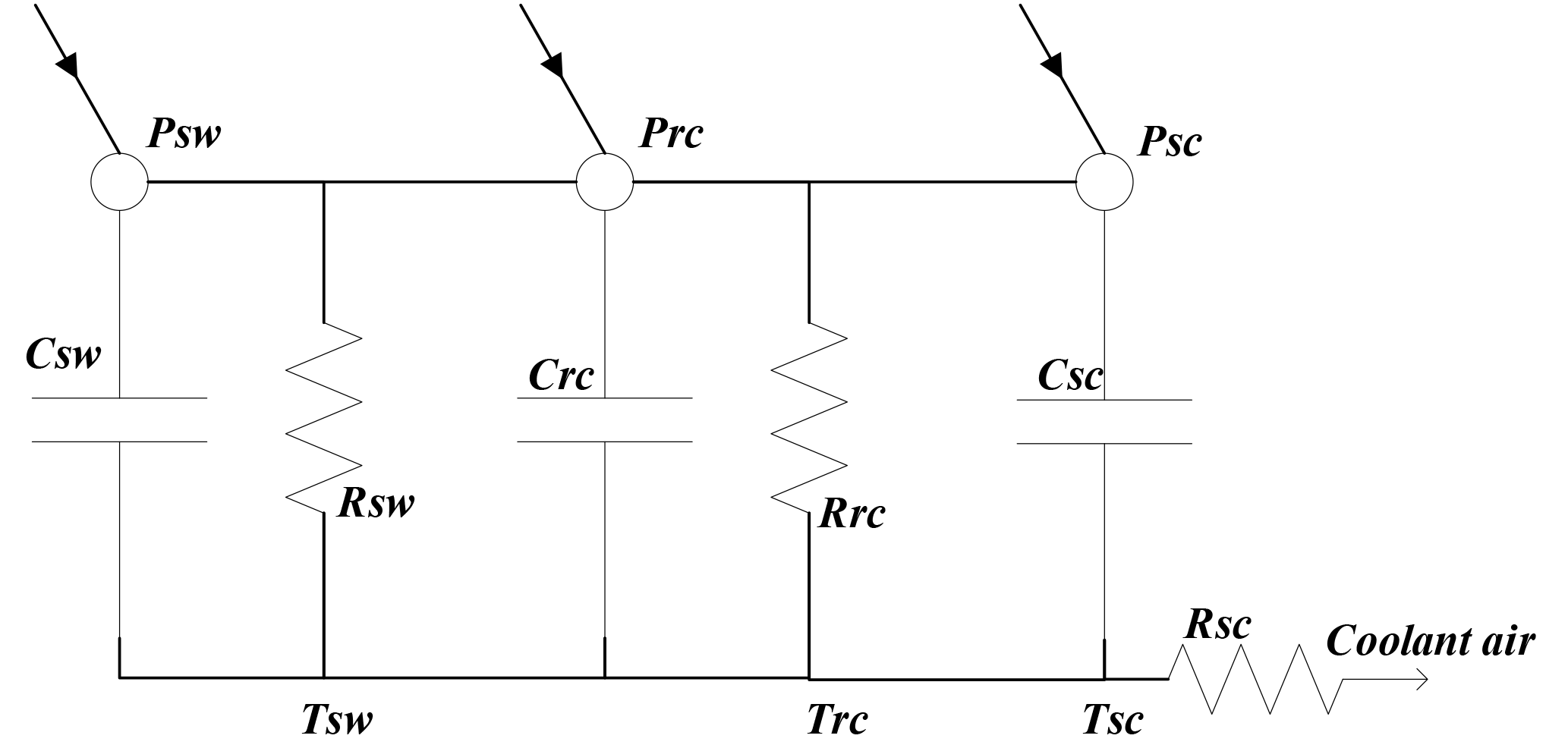
From the above figure, the state-space equations of the system are defined as the following equations:
where subscript sw indicates the stator winding, rc the rotor cage, sc the stator core and c the coolant air. ΔT is the temperature above ambient, R is the thermal resistance, C is the thermal capacitance and P is the power loss in the parts of the machine (indicated by the indices). The losses Psw, Prc, and Psc can be calculated from Eqs. (4) to (8).
In the simplified thermal model, Psw,Prc are ohmic loss, and Psc is the frequency-dependent iron loss, which are described in the paper by Haumer et al. (2009). Rs, Rr are the ohmic resistances, between any two line terminals, ωm is the mechanical speed of the rotor in rad s−1, and kiron is the iron loss constant.
As the currents of the rotor cage are not available to be measured or to be estimated using a simple method, the rotor cage losses can be calculated indirectly, which is defined by the IEEE Power Engineering Society (Society, 2004).
where Pin is the input power of the machine, and UL and IL are the line voltage and the line current, respectively. ωs is the synchronous speed, ωr is the rotor speed, and s is the slip of the machine.
The temperatures of the stator winding and rotor cage will increase largely. Normally it will be much higher than the reference ambient temperature. The rising temperature makes the resistance greater by more than 40 %. The electrical resistances will increase as the machine is running. So the ignored increasing temperature should be considered to calculate resistance, which is with respect to time. All in all, the stator winding loss can be calculated much more accurately than that of the constant value of the electrical resistance. Rs can be replaced by Eq. (9):
where RsRef is the stator winding resistance in the reference ambient temperature. αs is the temperature coefficient of the stator winding, with the value of 0.004041 1 K−1 for the copper.
The state-space equations of the system can be acquired by calculating the losses defined in Eqs. (4)–(5), and importing them into Eqs. (1)–(3). By summarizing the previous equations, the system can be rewritten as a fourth-order linear continuous time-variant system in the state-space model form:
where
In the state equations, x(t) is the state vector, u(t) is the control vector, A is the system transition matrix which is a constant matrix, and B is the input matrix which is also a constant matrix. In the measurement equation, C is the output matrix which is a constant in this system, and D is the feedthrough matrix which is zero here. The coolant air temperature Tc is considered a constant parameter due to the slow variation with time.
2.2 The target platform
The platform is the Preon32 wireless sensor node produced by Virtenio GmbH. It contains a 32-bit ARM Cortex-M3 micro-controller with 256 kB flash memory for programming and 64 kB RAM memory for data. A 2.4 GHz wireless transceiver which is compliant with the IEEE 802.15.4 standard can for example be used for ZigBee or 6LoWPAN communication. Two 12-bit analog-to-digital converters (ADCs) with a maximum sampling rate of 1 M samples/s are provided by the platform (Preon32, 2016). The clock for time keeping is generated from a low-power watch crystal and has a resolution of 2−14 s =61.035 µs and a width of 32 bit. The ADC of the Preon32 has a resolution of 12 bit and an input range of 0 …3.3 V. Its sampling period is derived from the CPU clock and can be set with a resolution of 1 µs (Funck and Guehmann, 2017).
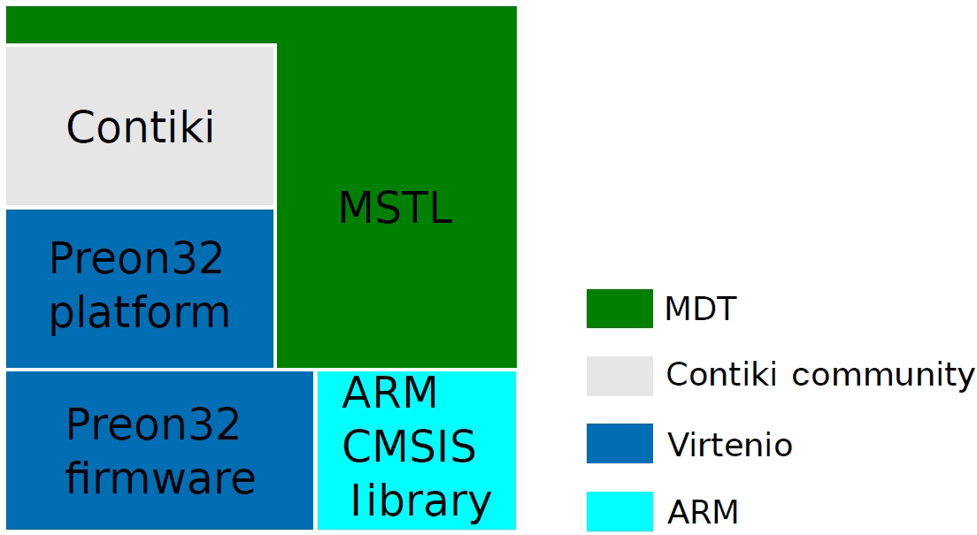
The whole software package is comprised as follows: Contiki, ARM CMSIS Library, Preon32 platform, Preon32 firmware and the MDT Smart Transducer Library (MSTL). Figure 2 shows the components of the WSN software. On the top layer of the Contiki MSTL, which is implemented by Jürgen Funck from the Chair of Electronic Measurement and Diagnostic Technology (MDT) of the Technical University of Berlin. It provides the management of the data acquisition for a variety of sensors and actuators of the wireless sensor nodes. It is inspired by the IEEE1451 family of standards for smart transducers.
2.3 Structure and topology of the system
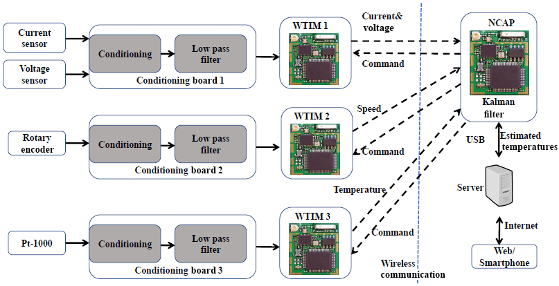
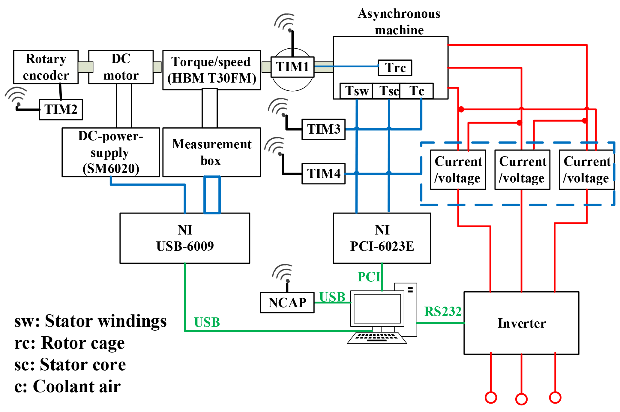
Based on the proposed KF algorithm, four types of signals are acquired as the inputs of the algorithm. Three Preon32 nodes are implemented as the WTIMs to acquire coolant air temperature, rotor speed, effective current and voltage. Data acquisition, data preprocessing and data transmission are performed by these WTIMs. Another node is implemented as the NCAP to receive the data from different WTIMs and to process the KF algorithm for temperature estimation. The structure of the temperature estimation system on WSN is shown in Fig. 3.
2.4 The hardware
Preon32 provides multiple I/O interfaces for connection to external peripheral digital I/O pins which could be used for the acquisition of rotor speed. Analog signals such as the coolant air temperature, the three-phase currents and voltages can be captured with the integrated ADC with a resolution of 12 bits and a possible sampling rate of up to 1 million samples per second. The conditioning boards were designed for connecting the sensors with Preon32 sensor nodes and conditioning the analog signal.
2.4.1 The conditioning board for three-phase currents and voltages
Six sensors based on the Hall effect for the three-phase currents and voltages are first mounted on a data acquisition board in the paper by Funck and Nowoisky (2011). An anti-aliasing filter is implemented to restrict the bandwidth of a signal to approximately satisfy the sampling theorem over the band of interest before signal acquisition. In order to scale the output voltages to the range of ±3.3 V, a conditioning board connecting to Preon32 was developed in a masters thesis (Hopp, 2013). They are shown in Figs. 4 and 5.


2.4.2 The conditioning board for coolant air temperature
The coolant air temperature is one of the inputs which should be measured and transmitted wirelessly by a Preon32 sensor node. Pt-1000 and a commercial conditioning board are used for the temperature acquisition. The output voltage of the conditioning board provided together with the sensor can be calibrated to the range of ±3.3 V.
2.4.3 The conditioning board for rotor speed
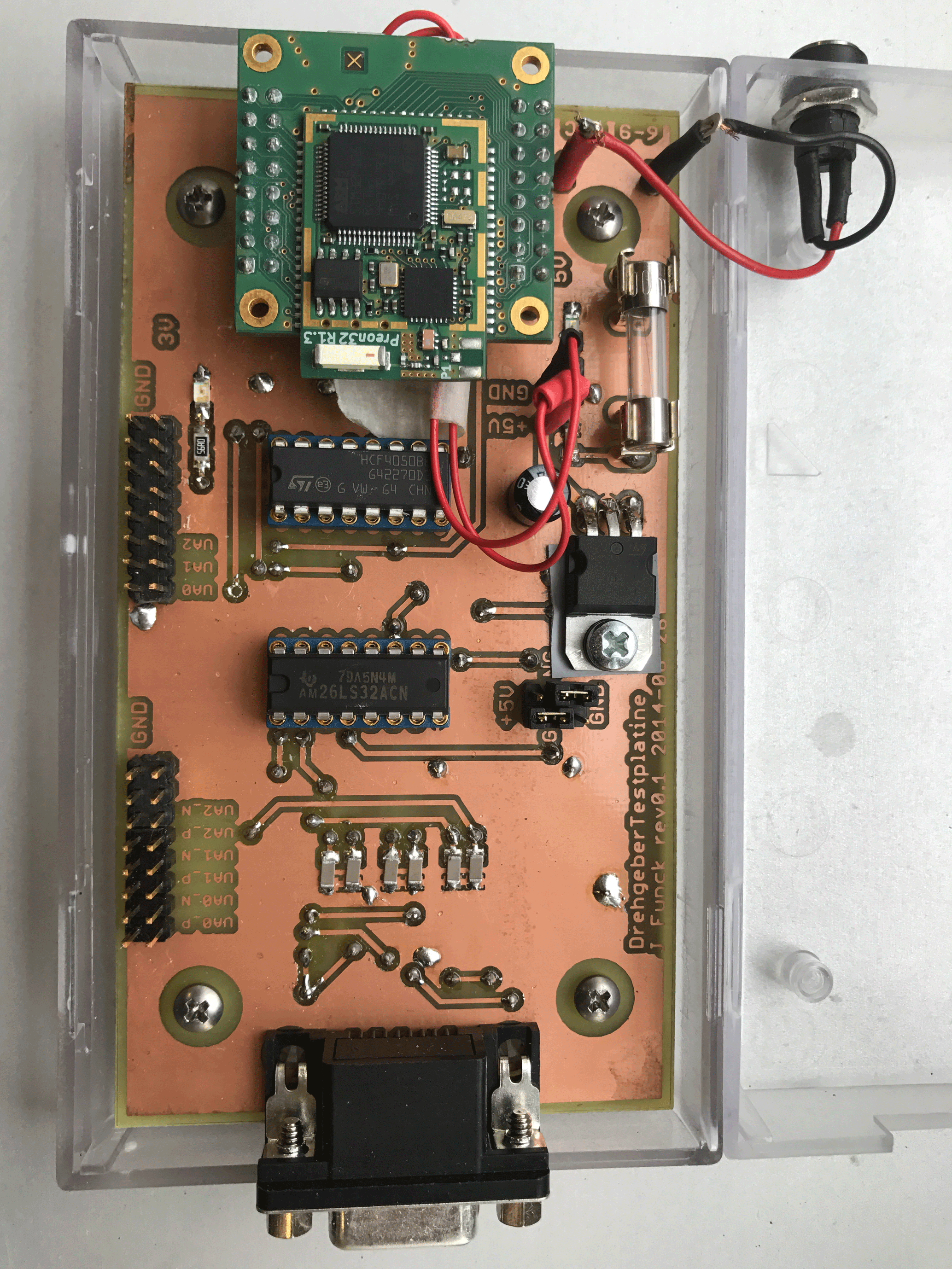
In order to acquire the speed of the rotor, a rotary encoder “ROD 426 B-6000” from HEIDENHAIN GmbH is used. A conditioning circuit board shown in Fig. 6 is designed by another project. The construction of the rotor speed acquisition system is shown in Fig. 7. A Preon32 sensor node is inserted on the board which is powered by 12 V and connected with the rotary encoder via a serial port.

The data acquisition system (DAQ) is implemented in WTIMs based on the MSTL which provides a universal interface to a variety of transducers. The implementation also follows the IEEE1451 family of standards in many places. The startTrigger or startStream commands are broadcasted from the NCAP to trigger the WTIMs simultaneously (IEE, 2007b). When WTIMs receive the command, data will be acquired periodically.
3.1 Analog sensor data acquisition
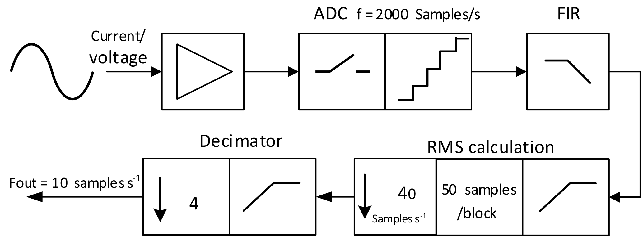
Hall sensors are mounted on the conditioning board with low-pass filters to process analog three-phase currents and voltages (Hopp, 2013). The Hamming window method is used for the FIR low-pass filter design, with the cutoff frequency of 120 Hz. The sampling rate is 2000 Hz. The instantaneous values of currents and voltages are acquired in a block once a second. The size of the block is 50 samples block−1. The effective values are used for loss calculation based on Eqs. (4)–(7). The average value of the coolant air temperature Tc is calculated once a second from the sampled and filtered signals. The frequency of the output values is decimated to 10 Hz. The values of the slope and intercept of the transformation equation of the sensors are stored in the TEDS (Transducer Electronic Data Sheet, IEE, 2007a), making it possible to transfer the values to SI units before transmission.
The measurement chain of the effective current and voltage is taken as an example to illustrate the measurement process, which is shown in Fig. 8. Firstly, three-phase analog currents and voltages are filtered by an anti-aliasing filter with the cut-off frequency of 100 Hz. Then analog signals are acquired and converted to digital signals with a sampling rate of 2000 Hz. A low-pass FIR filter is used to filter digital signals and to pass them for the RMS calculation. The effective value is calculated every 50 samples. In this way, the bandwidth is reduced such that it can be represented by 40 samples s−1. Another decimator is used to further reduce the signal bandwidth such that it can be represented by 10 samples s−1. The power consumption would be largely reduced due to the lower transmission frequency.
As data are acquired, filtered and transmitted continuously, the calculation time for each step must be considered. Buffers for data storage are allocated using MEMB memory block allocators, which is described in the documents (Allocation, 2016). On the other hand, the computation time of the filter must be shorter than the acquisition time for one filtered block. The detailed signal processing time division is shown in Fig. 9.

The total acquisition and conversion time for one block (sampling time Δt is 500 µs with 8 channels and 16 repetition counts, a total of 128 samples block−1) is µs. The total filtering and sending time is µs. As a result, the time of data acquisition is longer than the time of data processing, and the analog data acquisition system can process and transmit the data periodically from WTIM to the NCAP.
3.2 Digital sensor data acquisition
A rotary encoder (ROD 426B-6000) is mounted to the end of the machine shaft and connected to a conditioning board. A WTIM node is used to transfer the number of the pulse into the real rotor speed using etimer of Contiki. The acquisition of the generated pulses is shown in Fig. 10.

The rotation speed can be defined in Eq. (19), where τ is the time between two neighboring pulses, NLine counts is the number of encoder lines per revolution, and tsample is the time period in one session, which is 12∘ for the encoder.
3.3 Implementation of the processes in WTIMs
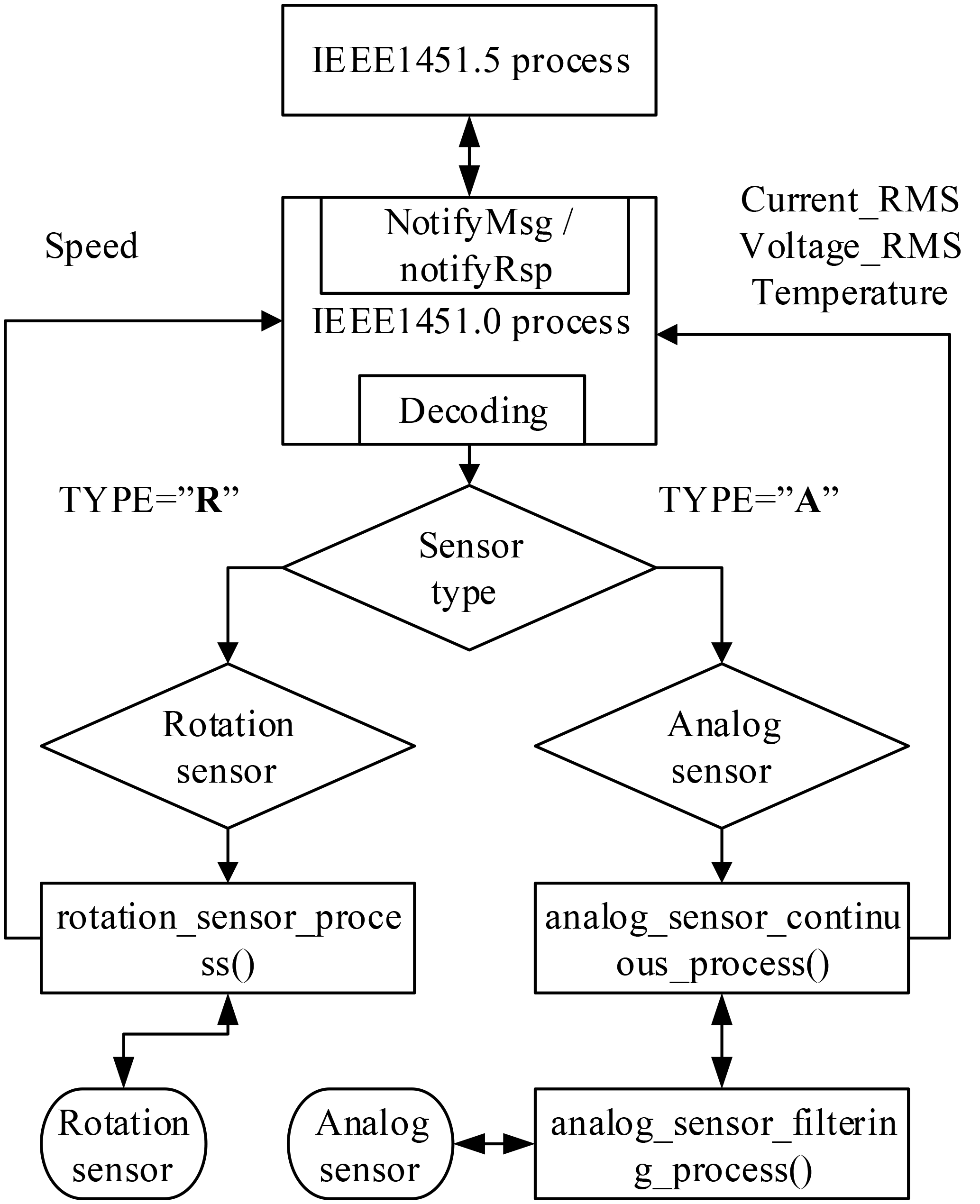
The general structure of the implemented WTIM is shown in Fig. 11. The IEEE1451.5 process is used to manage the radio module and to handle the communication of the WSN. The IEEE1451.0 process is used to manage the TEDS information and sample data of the sensors. It is a generic acquisition system for both rotation sensor and analog sensor, which is implemented in all the WTIMs. Which type of process to be used is determined by the sensor type in the command from the NCAP. The values acquired and processed by the acquisition system are sent back to the IEEE1451.0 process periodically as soon as the WTIM receives startTrigger or startStream commands. The values are stored in the package and sent back to the NCAP wirelessly via the IEEE1451.5 process.
This section discusses the implementation of the KF algorithm based on the IEEE1451 standard in the NCAP. The minimum implementation of the IEEE1451 standard has been integrated into both the WTIM and the NCAP. Sensors and actuators which are connected to the WTIM can be managed by wireless commands from the NCAP.
4.1 The Kalman filter algorithm
The Kalman filter is a set of mathematical equations that provides an efficient computational (recursive) means to estimate the state of a process, in a way that minimizes the mean of the squared error (Welch and Bishop, 1995). In general, both the process noise and the measurement noise should be taken into account in the system model and measurement model.
It is necessary to assume that the process wk and the measurement noise vk are independent of each other, a random white Gaussian noise with zero mean. Their variance can be described by the covariance matrix Q and R, respectively. The Kalman filter estimates a process by using a feedback control: the filter estimates the process state at some time and then obtains feedback in the form of (noisy) measurements (Welch and Bishop, 1995). As such, the equations of the Kalman filter can be divided into two groups: prediction equations and correction equations.
The prediction stage of the Kalman filter
The equations of the prediction stage shown in Eqs. (22) and (23) are responsible for projecting forward (in time) the current state and error covariance estimates to obtain a priori estimates for the next time step. Equation (22) is used for updating the state vector from previous sampling time k−1 to current time k. Equation (23) is the state of the updating error covariance matrix.
The discretization of the model
The model above is a continuous time system which cannot be processed by computer. Euler's approximation is used to discretize the model, so that the sampled data can be used in the KF algorithm. According to the definition of the derivative, Eq. (20) can be rewritten as
where and Bd=τB, E is a 4 × 4 unit matrix, Cd is equal to C, and τ is the sampling time.

The correction stage of the KF
The equations of the correction stage are responsible for the feedback – i.e., for incorporating a new measurement into a priori estimation to obtain an improved a posteriori estimation (Welch and Bishop, 1995).
where Kk is the Kalman gain and Hk is the measurement matrix.
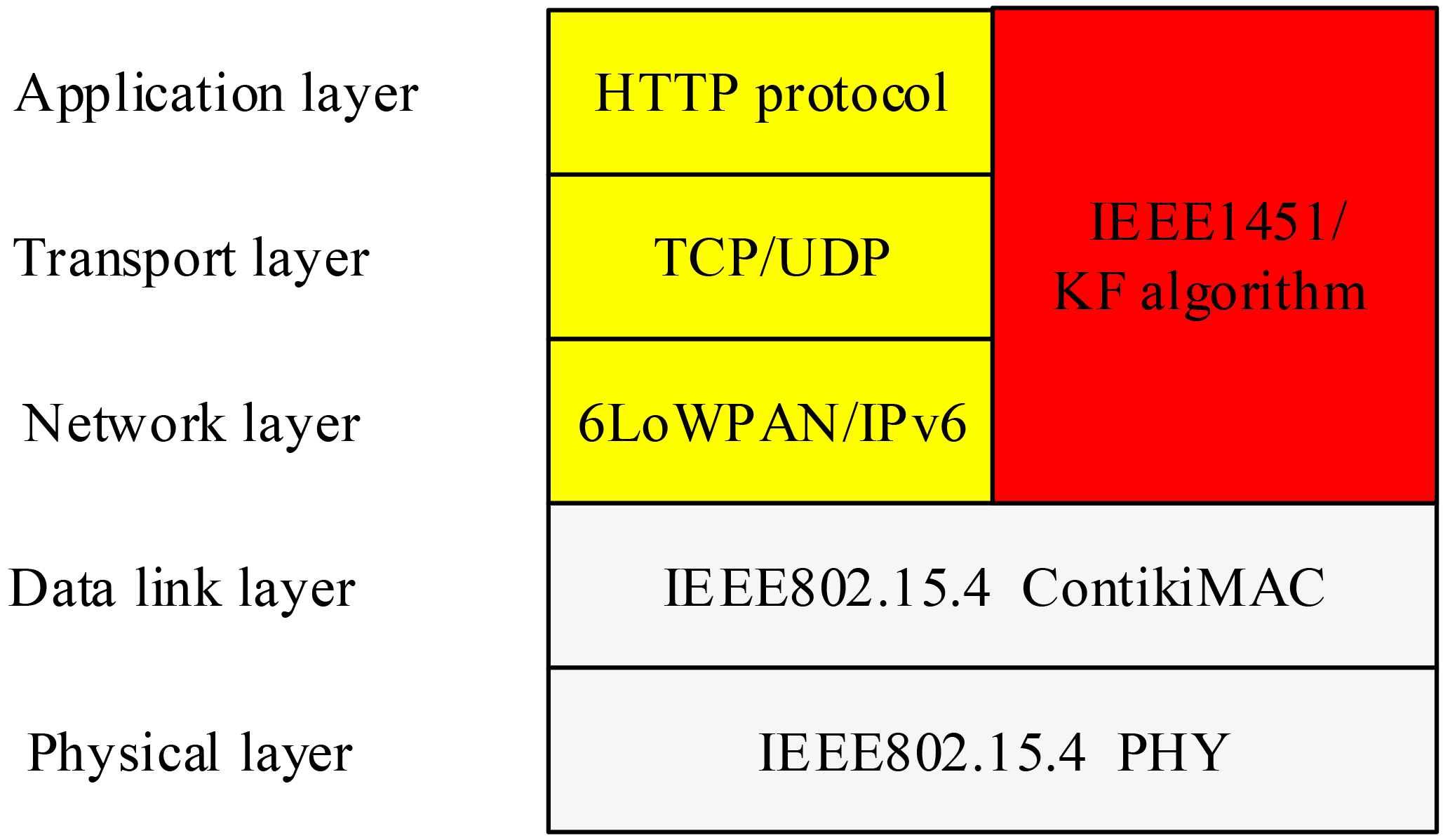
In our application, the KF algorithm is integrated into the NCAP to estimate the temperatures of stator windings, the rotor cage and the stator core of an induction machine. The Preon32 sensor node is resource restricted with respect to low costs, low power consumption and small memory size. In order to be implemented in the NCAP, the algorithm should be simple and efficient. The integration of the KF layer into the Contiki system stack is shown in Fig. 12.

6LoWPAN is defined encapsulation and header compression mechanisms that allow IPv6 packets to be sent to and received from IEEE802.15.4 links, whose full name is IPv6 over Low power Wireless Personal Area Networks (Shelby and Bormann, 2010). It is an adaptation layer of the Ipv6 protocol for WSN. The 6LoWPAN protocol has been implemented together with the IEEE802.15.4 Mac layer and IEEE802.15.4 PHY layer by Contiki OS. And the Transport layer is responsible for data transmission from an application layer between the client and server sides. In the application, IEEE1451.0 and IEEE1451.5 standards are implemented which are compatible with the stack. The KF algorithm is connected to the transport layer and application layer based on the API of the IEEE1451 standard. The efficiency of the messages is largely improved and the overhead of the IP address is reduced by using the header compression in the User Datagram Protocol (UDP). Users can manage the WTIM by sending the commands to the NCAP via the Internet, and the NCAP will send commands to WTIM for the information. All the API and commands are defined in the standard (IEE, 2007a, b).
4.2 KF algorithm implementation in the NCAP using fixed-point arithmetic
The KF algorithm is first implemented in MATLAB. It proved both in simulation and offline experiments on the test bench that the temperatures can be accurately estimated. In order to be implemented on the resource-restricted sensor node, the same KF algorithm is implemented in the C programming language using floating-point arithmetic on the Eclipse IDE platform. The workflow of the KF-Algorithm process is shown in Fig. 13, which can be summarized as follows: when kf_process starts, the system will retrieve and decode the messages from the messages_buffer where different messages from different WTIMs are stored. The function kf_data_gen() is then called to calculate the losses from the rotor speed and the preprocessed currents and voltages, and to generate the inputs with Tc. The inputs are stored in the structure kf_data and passed to the run_kf() function where the main Kalman filter process is performed. The DSP (Digital signal processing) library is used for the fixed-point matrix calculation. The state vector X and error covariance matrix P are stored in the structure kf_filter and sent back to the next recursion. The estimated temperatures Tsw, Trc, Tsc are sent out for storage and display. Tsw is sent back to calculate the losses of the stator winding so that the resistance rising due to temperature can be compensated.
Compared to the implementation in MATLAB and Eclipse in the C language, implementation on the Preon32 sensor node using Contiki OS faces several challenges.
Firstly, the methods to allocate and free memory space are different between the standard C library and Contiki OS. The standard C library allocates heap memory using the malloc() function. However, the Contiki platform specifies a small area of its memory space for the heap because of the resource restriction (Hopp, 2013). If the malloc() function is used for memory allocation, the heap could easily overflow. The MEMB memory block allocator is used to allocate a block of static memory to construct kf_data, which contains as the inputs for the algorithm. The structure kf_filter holds all the variables and matrixes which are used during the prediction stage and update stage of the KF algorithm.
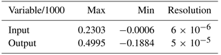
The second challenge is that the Preon32 does not have a floating-point unit. It is clear that the floating-point implementation cannot run online. As a result, fixed-point arithmetic is used for the implementation. In order to transfer the existing KF algorithm from floating-point to fixed-point representation, the proper Q format (Qm.n) defined in the document (Rein, 2008) has to be considered. Both the range and the resolution of the data are the key factors for choosing the type of Q format. The system can avoid computation overflow by the saturation modes provided by CPUs, or by designing the arithmetic operations. The number of overflow checks is minimized by the division of the variables by 1000, which scaled all the variables and auxiliaries to . By checking the computation in MATLAB step by step, the minimum value of a number is , which is larger than the Q1.31 format resolution. The data range and the resolution of variables are listed below in Table 1.
Thus the Q1.31 format is used for the arithmetic with a resolution of 2−31 and a range of . This means that one bit is used to designate the integer portion of the number, and the remaining 31 bits are used to designate the two's complement fractional part of the number (Rein, 2008).
The third challenge is the estimation time for every step. The ARM Cortex-M3 processor provides the CMSIS DSP library, which contains matrix functions in fixed point (CMSIS, 2016). These functions are optimized for checking the overflow and improving the calculation. By using these matrix functions in fixed-point arithmetic, the KF estimation time for every step (1 s step−1) is only 600 µs. As a result, online temperature estimation can be performed quite fluently.
4.3 The implementation of processes in the NCAP
Contiki OS is an event-driven system which is managed by protothreads. In order to operate different WTIMs, to manage the message transmission and to process the KF algorithm, several functional processes are implemented in the NCAP. The structure of the implemented processes is shown in Fig. 14.
Table 3Error and NRMSE of the estimated temperatures under S1.
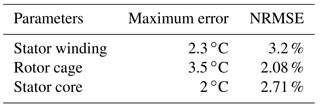
Table 4Error and NRMSE of the estimated temperatures under S6.
The Serial-Shell process is implemented for connecting the WSN to an arbitrary network. A PC connected to the NCAP works as a server of the network. Users can manage the WSN by using a web-based application or an App on a smartphone. The TIMDiscovery process is used first for discovering WTIMs before every command from the application process. The KF-Start process is used for configuring and initiating. The IEEE1451.5 process is implemented to manage the radio module and handle the data wireless transmission. The IEEE1451.0 process represents the interlayer between the IEEE1451.5 process and the KF-Start process. The buffer for storing data from different WTIMs is allocated in this process. The received will be passed to the KF-Algo process for the temperature estimation and the results will be sent out through the Serial-Shell process.
4.4 Memory usage and calculation time
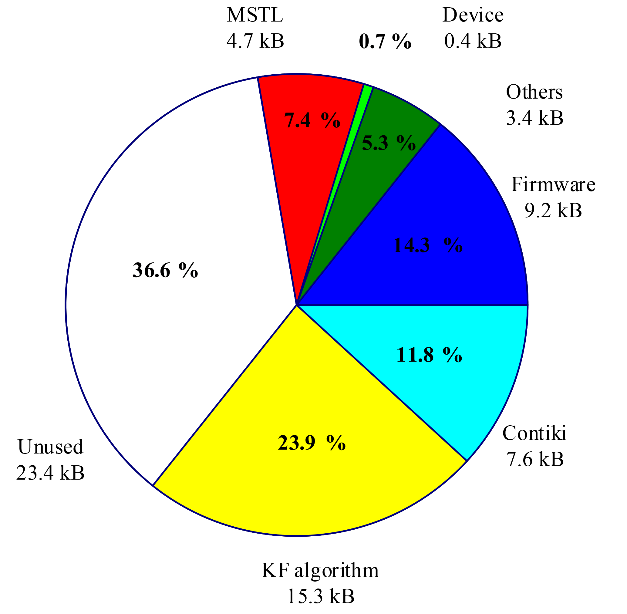
In the implementation of the KF algorithm in the NCAP, all the memory blocks are allocated statically so that fragmentation can be avoided (Haumer et al., 2012). By using this way, it is easy to analyze the memory usage of both RAM and Flash. The usage of RAM on the NCAP sensor node is shown in Fig. 15. The buffers of the KF algorithm take up about 24 % of the total memory space. The basic system, which consists of the Contiki OS, the firmware provided by Virtenio, and other parts from the standard C library, consumes about 32 %. The MSTL takes up 7.4 %. About 37 % of the space is unused.
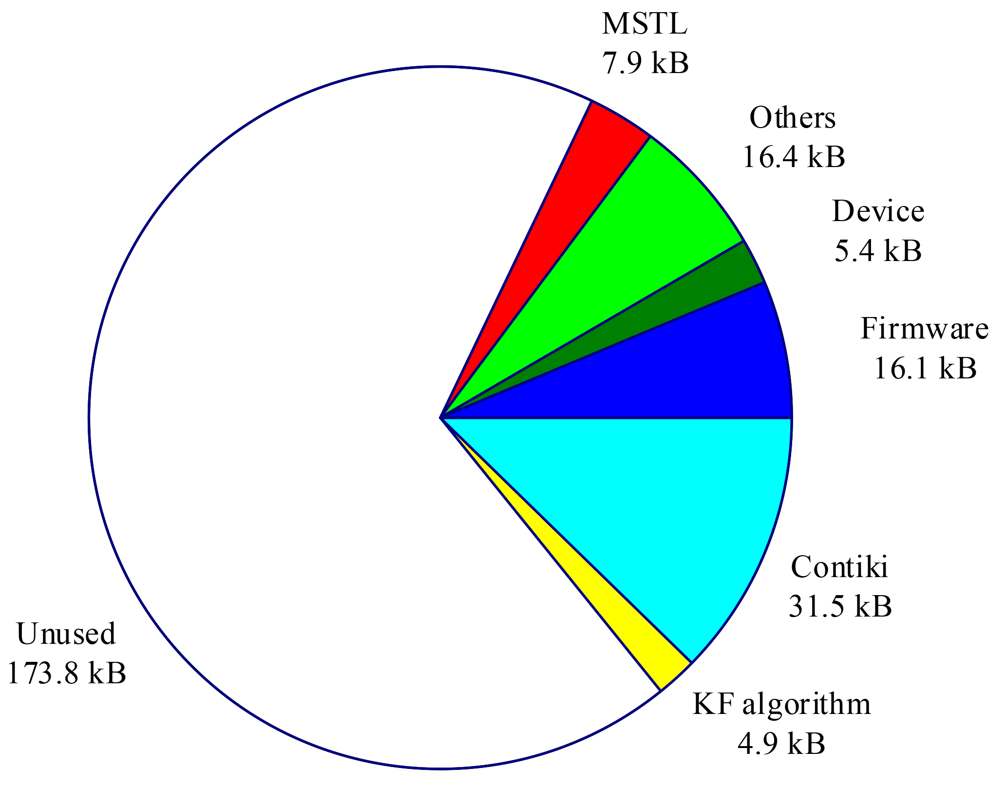
The usage of the flash memory for programming on the NCAP is shown in Fig. 16. Only about 5 % of the memory is used for the KF algorithm and the MSTL. The system takes up most of the used memory. The rest of about 62 % of the total memory is not used.
The system gets the data from different buffers to generate the input, which costs 120 µs, and the computation time of the KF algorithm for one step is about 600 µs. The total time of data generation and KF computation is much shorter than the calculation interval 1 s.
In the WSN system, the IEEE1451.5 standard defines the communication interfaces between the NCAP and WTIMs. The 6LoWPAN communication protocol is implemented in the network layer and UDP is used at the transport layer to comply with this specification in the standard.
5.1 Channel access method – the WSN system
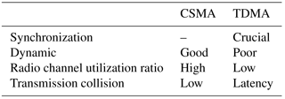
Three WTIMs continuously transmit data streaming to the NCAP. Radio channel collision, which is caused by two of the nodes sending data at the same time, is a great concern in the implementation. Carrier-sense multiple access (CSMA) and time-division multiple access (TDMA) are implemented in the MAC layer as the channel access methods, which can be selected according to different requirements of the application. The mechanism and the implementation of these two methods are out of the scope of this paper. Both CSMA and TDMA can be applied in this system through the experiment. Table 2 shows the comparison of these two channel access methods (Cionca et al., 2008).
CSMA prevents collisions by repeatedly detecting the channel and waiting for it to become available. So when a large number of nodes are operated in WSN with CSMA, the channel utilization is normally lower than with TDMA. When data from three different WTIMs are transmitted to the NCAP, collisions would happen or packages would be lost. Either of these events can influence the estimation results or block the process of the algorithm.
TDMA is an alternative mechanism to coordinate each node which is divided into time frames and each time frame is further divided into a fixed number of time slots. By using TDMA, data transmissions operate in a completely predictable way, which can largely reduce the collisions and almost prevent the packages from missing. Fewer collisions and more stable transmission have higher priority when determining channel access method. As a result, TDMA is used for this WSN system.
5.2 The sequence of the WSN system
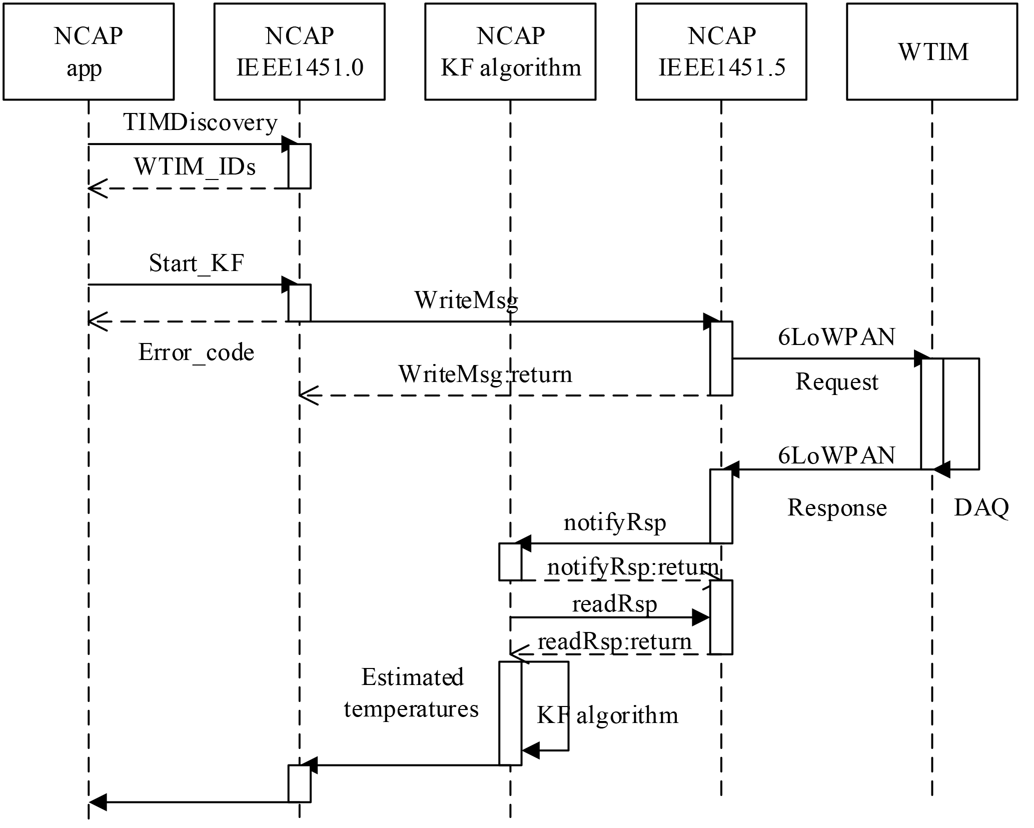
The sequence on the NCAP side is shown in Fig. 17. The TIMDiscovery command is first used to discover the available WTIMs in the network. After calling the start_KF function, the message is passed from the IEEE1451.0 layer to the IEEE1451.5 layer and then broadcasted to the WTIMs. Acquired data from different WTIMs are sent back to the NCAP and stored in a queue in different buffers which are identified by the WTIM_ID. The data from different buffers will be fetched by a data generation function according to the timestamps. Preprocessed data with the same or nearest timestamps will be passed and processed by the KF algorithm processed by the KF. Finally, the temperatures are estimated.
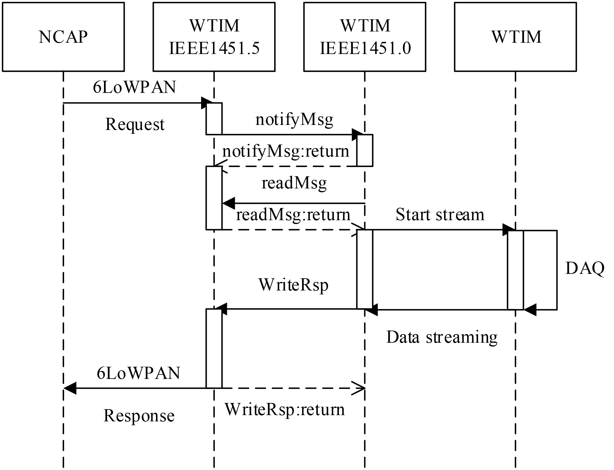
The sequence on the WTIM side is shown in Fig. 18. The message is notified and decoded by the IEEE1451.0 process. The data acquisition system can be triggered by the startStream command for continuous data acquisition. The DAQ is out of the scope of the IEEE1451 standard. The filtered and processed data are converted to the value in SI units and are sent back to the NCAP for the KF algorithm.
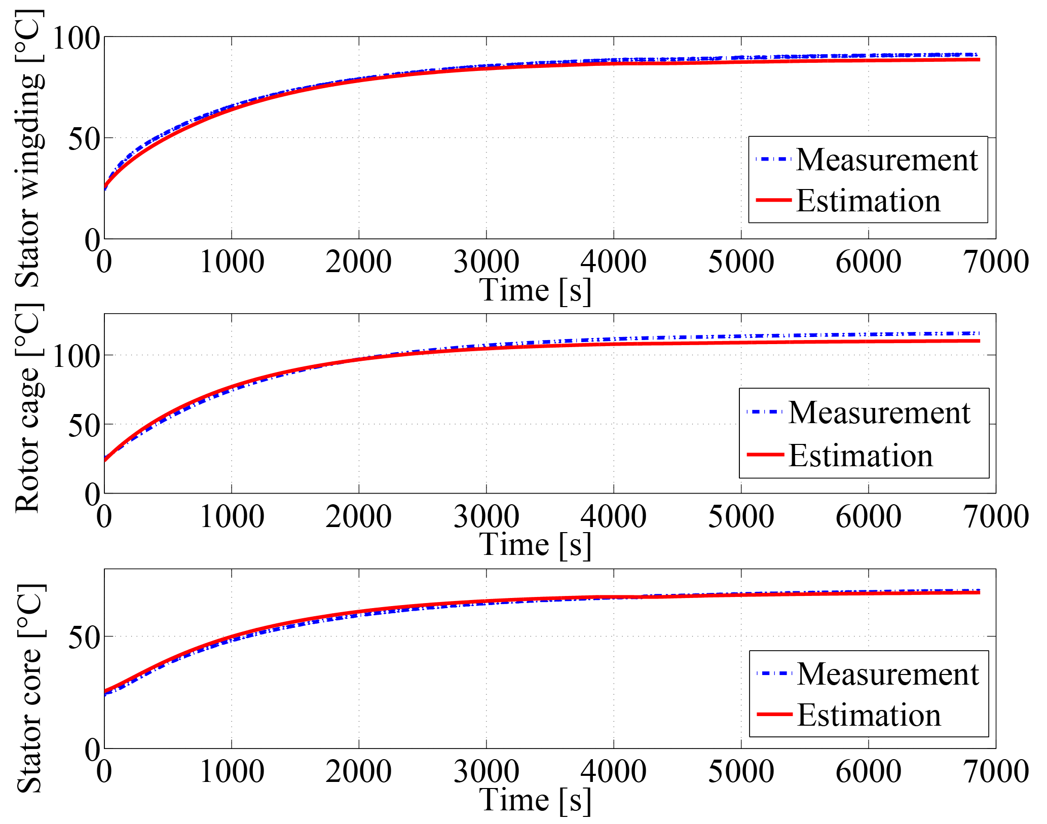
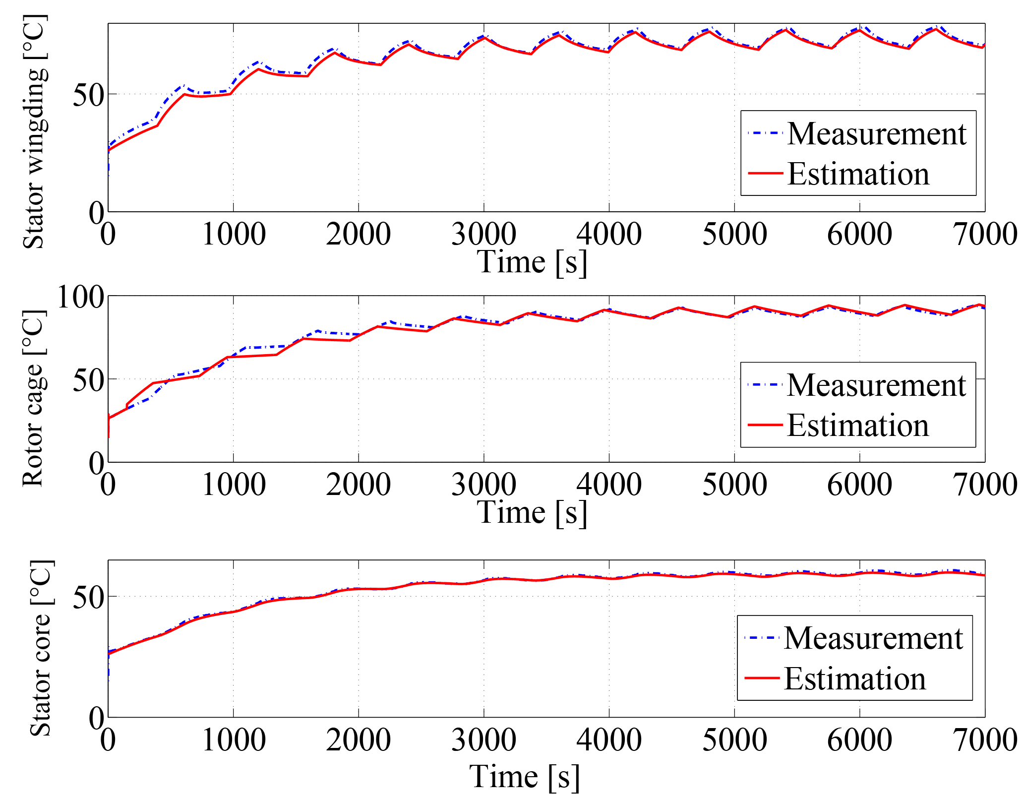
The structure of the test bench is shown in Fig. A1. Two experiments are performed on the test bench (Siemens machine: 1 LA5107-4AA20) using the WSN temperature estimation system. Wireless sensor nodes TIM2, TIM3 and TIM4 are used to acquire rotor speed, coolant air temperature, three-phase currents and voltages. The KF algorithm is implemented in the wireless sensor node as the NCAP to estimate the temperatures. The sampling time is 1 s. The sampling period is about 2 h, after which the temperatures of the estimated parts stay stable. The ambient temperature is 26 ∘C. The maximum errors and the normalized root-mean-square error (NRMSR) eNRMS defined in Eq. (30) are summarized in Table 3. The maximal deviation is 3.5 ∘C and the maximum NRMSR is 3.2 %. The comparisons of the estimated and measured temperatures under the continuous full-load test S1 condition are shown in Fig. 19.
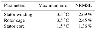
The other experiment under intermittent-load S6 (6 min no load followed by 4 min full load) is also performed on the test bench. The estimated and measured temperatures are shown in Fig. 20 and the maximum errors and NRMSE are listed in Table 4. The temperatures are estimated accurately under S6 with a maximum error of 3.5 ∘C, with the accuracy of 97 %. The difference may be due to the installation of PT1000 on the rotor cage, which influences the flux density and generates excessive losses (about 55 w) compared to a healthy machine (Bangura and Demerdash, 2000).
This paper describes the implementation of the temperature estimation system of induction machines on a WSN. The fourth-order KF with fixed-point arithmetic is implemented in the NCAP. Three WTIMs are implemented as the data acquisition systems. Compared to the floating-point implementation, the fixed point had the same estimation accuracy at only about one-fifth of the computation time. The KF algorithm is independent of the control strategy and the running conditions. That means no matter what the rotor speed is, and what the mechanical load is, as long as there are currents through the stator winding, the temperature can be estimated correctly. The experiments prove that the KF implementation is suitable for real-time temperature estimation on a resource-limited wireless sensor node. If wireless transmission has collapsed or packages are missing, the system can be rebooted for temperature estimation.
The underlying research data are stored in an internal system. All measurement data are not publicly available and can be accessed from the authors upon request.
The authors declare that they have no conflict of interest.
This article is part of the special issue “Sensor/IRS2 2017”. It is a result of the AMA Conferences, Nuremberg, Germany, 30 May–1 June 2017.
I would like to express my appreciation to my doctoral thesis advisor, Clemens Gühmann, who kept giving me
invaluable guidance for the research. I would like to thank my colleague, Jürgen Funck, and my student Wenjun Zhu for their help.
Edited by: Andreas König
Reviewed by: three anonymous referees
Allocation: Memory allocation, available at: https://github.com/contiki-os/contiki/wiki/Memory-allocation, last access: 15 June 2016. a
Bangura, J. F. and Demerdash, N. A.: Effects of broken bars/end-ring connectors and airgap eccentricities on ohmic and core losses of induction motors in ASDs using a coupled finite element-state space method, IEEE T. Energy Conver., 15, 40–47, https://doi.org/10.1109/60.849114, 2000. a
Ben Brahim, S., Bouallegue, R., David, J., Vuong, T. H., and David, M.: A Wireless On-line Temperature Monitoring System for Rotating Electrical Machine, Wireless Personal Communications, 1–21, https://doi.org/10.1007/s11277-016-3808-5, 2016. a
Brahim, S. B., Bouallegue, R., David, J., and Vuong, T. H.: Modelling and characterization of rotor temperature monitoring system, in: 2016 International Wireless Communications and Mobile Computing Conference (IWCMC), 735–740, https://doi.org/10.1109/IWCMC.2016.7577148, 2016. a
Cionca, V., Newe, T., and Dadaerlat, V.: TDMA Protocol Requirements for Wireless Sensor Networks, in: 2008 Second International Conference on Sensor Technologies and Applications (sensorcomm 2008), 30–35, https://doi.org/10.1109/SENSORCOMM.2008.69, 2008. a
CMSIS: CMSIS – Cortex Mircrocontroller Software Interface Standard, avaiable at: http://www.keil.com/pack/doc/CMSIS/General/html/index.html, last access: 20 June 2016. a
Funck, J. and Guehmann, C.: A flexible filter for synchronous angular resampling with a wireless sensor network, Measurement, 98, 393–406, https://doi.org/10.1016/j.measurement.2016.07.062, 2017. a
Funck, J. and Nowoisky, S.: MDT Strom- und Spannungswandler-Modul, unpublished, 2011. a
Haumer, A., Kral, C., Kapeller, H., Baeuml, T., and Gragger, J. V.: The AdvancedMachines library: Loss models for electric machines, in: Proceedings of the 7th Modelica Conference, 847–854, 2009. a
Haumer, A., Kral, C., Vukovic, V., David, A., Hettfleisch, C., and Huzsvar, A.: A Parametrization Scheme for High Performance Thermal Models of Electric Machines using Modelica, Proceedings of the 7th Vienna Conf. on Math. Modeling, Vienna, Austria, 15–17 February 2012. a, b, c
Hopp, T.: Intelligenter Sensor zur Leistungsmessung im Dreiphasennetz, MS thesis, Technische Universitaet Berlin, 2013. a, b, c
Hudon, C., Guddemi, C., Gingras, S., Leite, R. C., and Mydlarski, L.: Rotor temperature monitoring using fiber Bragg gratings, in: 2016 IEEE Electrical Insulation Conference (EIC), 456–459, https://doi.org/10.1109/EIC.2016.7548636, 2016. a
IEEE: Standard for a Smart Transducer Interface for Sensors and Actuators – Common Functions, Communication Protocols, and Transducer Electronic Data Sheet (TEDS) Formats, IEEE Std 1451.0-2007, 1–335, https://doi.org/10.1109/IEEESTD.2007.4338161, 2007a. a, b, c
IEEE: Standard for a Smart Transducer Interface for Sensors and Actuators Wireless Communication Protocols and Transducer Electronic Data Sheet (TEDS) Formats, IEEE Std 1451.5-2007, C1–236, https://doi.org/10.1109/IEEESTD.2007.4346346, 2007b. a, b
Ozsoy, E., Gokasan, M., and Bogosyan, S.: Simultaneous rotor and stator resistance estimation of squirrel cage induction machine with a single extended kalman filter, Turk. J. Electr. Eng. Co., 18, 853–864, 2010. a
Preon32: Datasheet Preon32, available at: http://www.virtenio.com/en/products/radio-module.html (last access: 25 November 2015), 2016. a
Rein, S.: Fixed-Point Arithmetic in C: A Tutorial and an Example on Wavelet Filtering, unpublished, 2008. a, b
Sabaghi, M., Farahani, H. F., Hafezi, H. R., Kiani, P., and Jalilian, A. R.: Stator winding resistance estimation for temperature monitoring of induction motor under unbalance supplying by DC injection method, in: Universities Power Engineering Conference, 2007, UPEC 2007. 42nd International, 217–222, https://doi.org/10.1109/UPEC.2007.4468949, 2007. a
Shelby, Z. and Bormann, C.: 6LoWPAN: The Wireless Embedded Internet, Wiley Publishing, 2010. a
Society: IEEE Standard Test Procedure for Polyphase Induction Motors and Generators, ISBN: 0-7381-3977-7 SH95211, 2004. a
Sonnaillon, M. O., Bisheimer, G., Angelo, C. D., and García, G. O.: Online Sensorless Induction Motor Temperature Monitoring, IEEE T. Energy Conver., 25, 273–280, https://doi.org/10.1109/TEC.2010.2042220, 2010. a
Wang, L., Yang, X., and Sheng, B.: Distributed Optical Fiber Sensor for Virtual Monitoring of Turbine Rotor's Temperature, in: 2009 International Conference on Measuring Technology and Mechatronics Automation, 1, 16–19, https://doi.org/10.1109/ICMTMA.2009.215, 2009. a
Welch, G. and Bishop, G.: An Introduction to the Kalman Filter, Tech. rep., Chapel Hill, NC, USA, 1995. a, b, c
- Abstract
- Introduction
- The system description
- Implementation of the data acquisition system in distributed WTIMs
- Implementation of the Kalman filter algorithm in the NCAP
- The communication of the WSN system
- Experiments
- Conclusions
- Data availability
- Appendix A
- Competing interests
- Special issue statement
- Acknowledgements
- References